Sigma-Weighted Fitting
Synthetic example
The fixture below is a single seeded peak with a known, deliberately
heteroscedastic per-point uncertainty profile — chosen to demonstrate
that supplying sigma changes both the fit and the covariance formula
used, not a sweep proving this across real measurement-noise models.
Quick example
Per-point measurement uncertainty is known and heteroscedastic — noise that
scales with the signal itself, as in counting statistics. Pass it as sigma
on MeasurementData so the fit weights each point by its actual reliability
instead of trusting every point equally.
def synthesize_data() -> tuple[np.ndarray, np.ndarray, np.ndarray]:
    """Synthesize a peak on a background with Poisson-like, signal-scaled noise.

    ``sigma_i = sqrt(signal_i) * NOISE_SCALE`` mimics counting statistics:
    the low-signal baseline is comparatively quiet, the high-signal peak
    apex is comparatively noisy. Returns ``(x, y, sigma_true)`` — the true
    per-point sigma is normally not directly known, but here it is exactly
    what was used to draw the noise, so it can be passed to the weighted fit
    below as if it came from an independent noise model (e.g. a detector's
    counting-statistics calibration).
    """
    rng = np.random.default_rng(3)
    x = np.linspace(-3, 3, 100)
    signal = BACKGROUND_TRUE + AMPLITUDE_TRUE * np.exp(
        -0.5 * ((x - CENTER_TRUE) / SIGMA_TRUE) ** 2,
    )
    sigma_true = np.sqrt(signal) * NOISE_SCALE
    noise = rng.normal(0, 1, len(x)) * sigma_true
    y = signal + noise
    return x, y, sigma_true


x, y, sigma_true = synthesize_data()
sigma_i = sqrt(signal_i) * NOISE_SCALE mimics counting statistics: the
low-signal baseline is comparatively quiet, the high-signal peak apex is
comparatively noisy. The same peak-plus-background graph is fit against
both variants of the data below.
def build_graph() -> FitGraph:
    """One Gaussian peak + one constant background node (both models fit this)."""
    return FitGraph(
        nodes=[
            ModelNodeSpec(
                id="peak",
                model_type=ModelType.GAUSSIAN,
                parameters={
                    "amplitude": Parameter(value=20.0),
                    "center": Parameter(value=0.0),
                    "sigma": Parameter(value=0.5, min=1e-3),
                },
            ),
            ModelNodeSpec(
                id="bg",
                model_type=ModelType.CONSTANT,
                parameters={"c": Parameter(value=1.0)},
            ),
        ],
    )
The only difference between the two fit() calls is whether sigma is
attached to MeasurementData — data_unweighted omits it entirely, so
every point is treated as equally reliable regardless of where it sits on
the signal-scaled noise curve.
def fit_both(
    x: np.ndarray,
    y: np.ndarray,
    sigma_true: np.ndarray,
) -> dict[str, FitResult]:
    """Fit once with ``sigma=None`` (uniform weighting), once with the true sigma."""
    data_unweighted = MeasurementData(x=x.tolist(), y=y.tolist())
    data_weighted = MeasurementData(
        x=x.tolist(),
        y=y.tolist(),
        sigma=sigma_true.tolist(),
    )
    return {
        "unweighted": fit(build_graph(), data_unweighted),
        "weighted": fit(build_graph(), data_weighted),
    }


results = fit_both(x, y, sigma_true)
unweighted_result, weighted_result = results["unweighted"], results["weighted"]
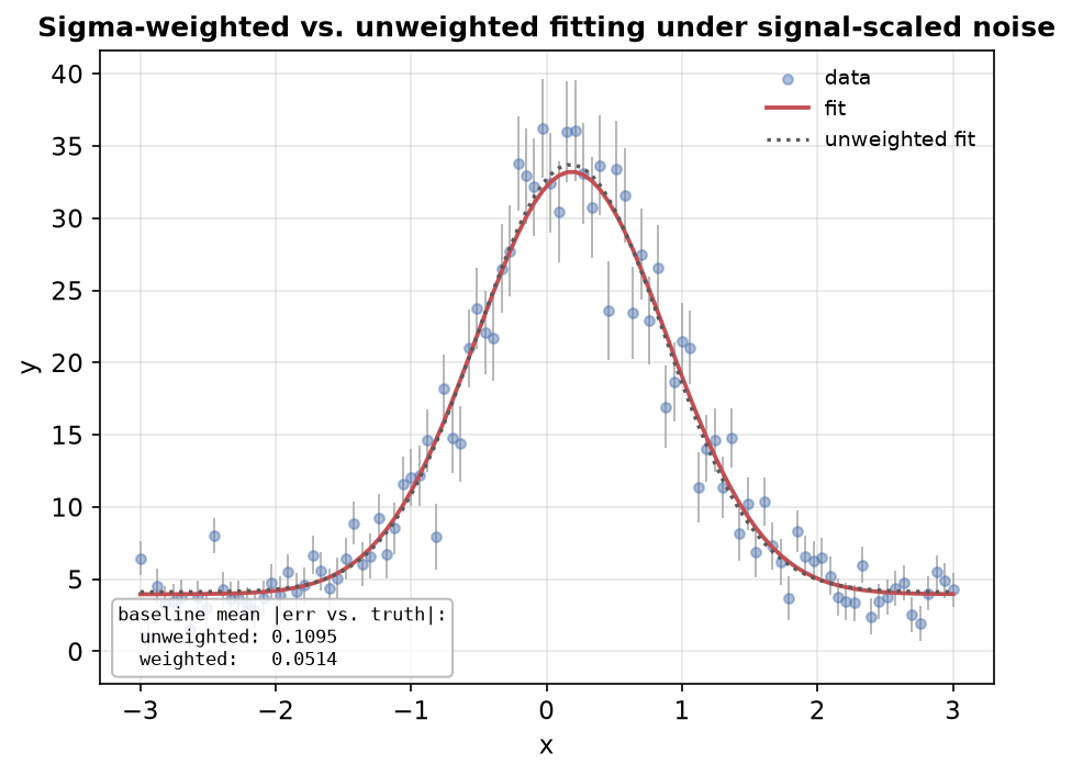
Comparing both fits against the true noiseless model — not just against the noisy data — is what turns "weighting should help" into a checked number: the mean absolute deviation from truth in the low-signal baseline region, where the weighted fit's trust in those quieter points should show up as a tighter fit.
def compare(
    x: np.ndarray,
    unweighted_result: FitResult,
    weighted_result: FitResult,
) -> tuple[float, float]:
    """Compare both fits against the true noiseless model in two x-regions.

    ``baseline_mask`` picks points far from the peak (low true signal, low
    true sigma); ``peak_mask`` picks points near the apex (high true signal,
    high true sigma). Returns the mean absolute deviation from the true
    model in the baseline region for ``(unweighted, weighted)`` — the
    concrete number backing the claim that the weighted fit tracks the
    low-noise region more tightly, since it correctly discounts the noisier
    high-signal points instead of treating them as equally trustworthy.
    """
    true_model = BACKGROUND_TRUE + AMPLITUDE_TRUE * np.exp(
        -0.5 * ((x - CENTER_TRUE) / SIGMA_TRUE) ** 2,
    )
    baseline_mask = np.abs(x - CENTER_TRUE) > 2 * SIGMA_TRUE
    err_unweighted = np.abs(np.array(unweighted_result.best_fit) - true_model)
    err_weighted = np.abs(np.array(weighted_result.best_fit) - true_model)
    baseline_err_unweighted = float(err_unweighted[baseline_mask].mean())
    baseline_err_weighted = float(err_weighted[baseline_mask].mean())

    print(f"{'':12s} {'amplitude':>10s} {'stderr':>10s} {'baseline |err|':>16s}")
    for name, result, baseline_err in (
        ("unweighted", unweighted_result, baseline_err_unweighted),
        ("weighted", weighted_result, baseline_err_weighted),
    ):
        amp = result.parameters["peak.amplitude"]
        print(f"{name:12s} {amp.value:10.4f} {amp.stderr:10.4f} {baseline_err:16.4f}")

    assert unweighted_result.success
    assert weighted_result.success
    assert baseline_err_weighted < baseline_err_unweighted, (
        "the weighted fit should track the low-noise baseline more tightly "
        "than the unweighted fit on this seeded example"
    )
    return baseline_err_unweighted, baseline_err_weighted


baseline_err_unweighted, baseline_err_weighted = compare(
    x,
    unweighted_result,
    weighted_result,
)
Why this works
Distinct from confidence_intervals.md: that page derives output
uncertainty (stderr → a confidence interval) from the Jacobian, always
under uniform per-point weighting. This example supplies input per-point
uncertainty that changes both what the solver minimizes and which of two
covariance formulas it uses to report stderr. Solver — Post-fit
statistics
documents both paths: without sigma, \(\mathrm{cov} = (J^T J)^{-1} \cdot (\chi^2 / \mathrm{dof})\) — a
scale-from-residuals estimate assuming uniform reliability; with sigma,
\(\mathrm{cov} = (J_w^T J_w)^{-1}\) where \(J_w[i, :] = J[i, :] / \sigma_i\) — the Jacobian itself
is weighted by each point's uncertainty before the covariance is formed.
Note that the reported chi2 is always the same unweighted sum-of-squares
either way — sigma changes the optimization and the stderr formula, not
how chi2 is reported. Both covariance formulas are still the same
Jacobian-based linear approximation around the fitted optimum that
Confidence Intervals flags — weighting by sigma
changes which quadratic form is estimated, not whether it's still only a
local approximation, and stderr can still be None under either path if
the (weighted) Jacobian is ill-conditioned.
What just happened
-
Data creation — a Gaussian peak on a constant background, with noise whose standard deviation scales as
sqrt(signal)— quiet baseline, noisier peak apex. -
Two fits, one graph shape —
fit_both()callsfit()once withsigma=None(uniform weighting) and once with the true per-pointsigmaattached toMeasurementData. -
Weighted fit tracks the low-noise region more tightly — measured against the true noiseless model, the weighted fit's mean absolute error in the baseline region is smaller than the unweighted fit's on this seeded example, since it correctly discounts the noisier high-signal points instead of pulling toward them as if they were equally reliable.
-
Different
stderr, samechi2reporting convention — the two fits'amplitude.stderrdiffer because they come from the two distinct covariance formulas described above; the printedchi2for both is the same unweighted sum-of-squares convention regardless ofsigma.
See also
- Related examples:
confidence_intervals.md(turningstderrinto a 95% CI, always under uniform weighting),fitting.md(the unweighted baseline case). - Reference: Solver — Post-fit statistics.
- API docs:
MeasurementData,FitResult,ParameterResult.