N-Dimensional (≥3-D) Fitting¶

Synthetic examples

All examples below are synthetic and illustrative — a single seeded geometry each, chosen to demonstrate the mechanism, not measured data and not a sweep that proves accuracy across all problem sizes, models, or noise levels.

Native N-D example — one 3-D Gaussian¶

You have a genuinely N-dimensional dataset — spectral intensity over (x, y, z) coordinates, or (kx, ky, kz, energy) — and want to fit one model jointly across all dimensions (e.g. a trivariate Gaussian).

def _synthesize_3d_gaussian() -> tuple[
    np.ndarray,
    np.ndarray,
    tuple[float, ...],
    tuple[float, ...],
]:
    """Sample a noisy 3-D Gaussian on an 8x8x8 grid.

    Returns:
        ``(coords, y, center, sigma)`` where ``coords`` has shape ``(512, 3)``,
        ``y`` has shape ``(512,)``, and ``center``/``sigma`` are the true
        (planted) parameter values used to generate the data.
    """
    n = 8
    g = np.linspace(-5.0, 5.0, n)
    xx, yy, zz = np.meshgrid(g, g, g, indexing="ij")
    coords = np.column_stack([xx.ravel(), yy.ravel(), zz.ravel()])  # (512, 3)

    amp, center, sigma = 6.0, (-1.5, 1.0, 0.5), (1.6, 2.1, 1.2)
    rng = np.random.default_rng(7)
    y = amp * np.exp(
        -((xx - center[0]) ** 2) / (2 * sigma[0] ** 2)
        - ((yy - center[1]) ** 2) / (2 * sigma[1] ** 2)
        - ((zz - center[2]) ** 2) / (2 * sigma[2] ** 2),
    ) + rng.normal(0.0, 0.05, xx.shape)

    return coords, y.ravel(), center, sigma


coords, y, true_center, true_sigma = _synthesize_3d_gaussian()

With a genuinely 3-D coordinate cloud in hand, the model needs one node whose parameters are indexed per axis (center_0..center_2, sigma_0..sigma_2) rather than three separate center/sigma params — that's what lets the compiler infer D=3 from the parameters supplied instead of you declaring a dimension anywhere.

def _build_graph() -> FitGraph:
    """Build a single ``gaussian_nd`` node. D=3 is inferred from center_0..2.

    No dimension field is passed anywhere -- the compiler counts the
    ``center_<i>`` parameters supplied below and validates the full
    ``1 + 2*D`` parameter set is present.
    """
    return FitGraph(
        nodes=[
            ModelNodeSpec(
                id="g",
                model_type=ModelType.GAUSSIAN_ND,
                parameters={
                    "amplitude": Parameter(value=4.0),
                    "center_0": Parameter(value=-1.0),
                    "center_1": Parameter(value=0.5),
                    "center_2": Parameter(value=0.0),
                    "sigma_0": Parameter(value=1.0, min=1e-3),
                    "sigma_1": Parameter(value=1.0, min=1e-3),
                    "sigma_2": Parameter(value=1.0, min=1e-3),
                },
            ),
        ],
    )

"D is inferred" matters at solve time too: this is one simultaneous least-squares problem over all 512 points, with the executor striding the flat coordinate buffer by D and the analytic Jacobian covering every axis at once — not three independent 1-D fits stitched together.

def fit_and_report(
    coords: np.ndarray,
    y: np.ndarray,
    true_center: tuple[float, ...],
    true_sigma: tuple[float, ...],
) -> tuple[FitResult, list[float]]:
    """Run the joint 3-D least-squares solve and print the per-axis report.

    One simultaneous fit over all 512 points -- the executor strides the
    flat coordinate buffer by ``D=3`` and the analytic Jacobian covers every
    axis, so this is never decomposed into three independent 1-D fits.

    Returns:
        ``(result, fitted_center)`` -- the raw ``FitResult`` and the fitted
        ``[center_0, center_1, center_2]`` values (as a plain list), which
        the ``__main__`` plotting block needs to pick projection slices.
    """
    graph = _build_graph()
    data = MeasurementData(x=coords.tolist(), y=y.tolist())
    result = fit(graph, data)

    print(f"Success: {result.success}   R²: {result.r_squared:.6f}")
    p = {k: v.value for k, v in result.parameters.items()}
    fitted_center: list[float] = []
    for i in range(3):
        center_i = p[f"g.center_{i}"]
        fitted_center.append(center_i)
        print(
            f"  axis {i}: center={center_i:+.3f} (true {true_center[i]:+.1f}), "
            f"sigma={p[f'g.sigma_{i}']:.3f} (true {true_sigma[i]:.1f})",
        )

    return result, fitted_center


result, fitted_center = fit_and_report(coords, y, true_center, true_sigma)

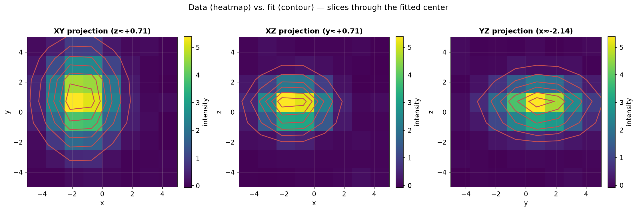
Why this works¶

As of SP-2, spectrafit fits this natively: the parametric gaussian_nd kernel handles any dimensionality D, and the dimensionality is inferred from the node's indexed center_<i> parameters. No MeasurementData3D class is needed — a D-dimensional point is just a coordinate row of length D.

Shared-model global fit

If instead you have several datasets sharing one model (e.g. spectra at different conditions, each with its own amplitude but a shared peak shape), that is a shared-model global fit — use GlobalFitGraph; see the "Stacked slices" alternative below and multi_dataset.md.

Arbitrary N (demonstrated at 3-D and 5-D)¶

gaussian_nd is not capped at 3-D. Give it center_0..center_4 / sigma_0..sigma_4 and a 5-D coordinate grid, and it fits a 5-D Gaussian the same way — the kernel and the solver are structurally dimensionality-general (the kernel sums over all D axes; the executor strides by D), so there is no dimension-specific code path that caps N. That structural generality is demonstrated at 3-D and 5-D by the Rust solver tests (run_gaussian_nd_recovery at d=3 and d=5); higher N follows from the same code path but is not separately accuracy-tested here. The only practical limit is that an N-D grid has points = size**N, so keep per-axis resolution modest at high N.

What just happened¶

Data — a synthetic 3-D Gaussian sampled with light noise (\(\sigma=0.05\)).
Graph — a single gaussian_nd node. Its parameters are indexed (center_0..center_{D-1}, sigma_0..sigma_{D-1}, plus amplitude); the compiler counts the center_<i> parameters to infer D=3 and validates the full 1 + 2D set is present (a missing center_i raises a clear error).
Fit — one simultaneous least-squares solve over all 512 points. The executor strides the flat coordinate buffer by D, and the analytic Jacobian covers every axis. The planted center/\(\sigma\) are recovered to within a few percent.

Performance note¶

The N-D path evaluates the model per point (the optimized batched fast-path is 1-D-only), so very large N-D grids (size**N points) are heavier than a 1-D fit of the same point count. For volumetric data, keep the per-axis resolution modest, or down-sample before fitting.

Alternative — stacked slices (different parameters per slice)¶

If your "third dimension" is really an index over datasets that share a model but differ per slice (e.g. a Gaussian whose amplitude changes from slice to slice while center/\(\sigma\) stay fixed), that is a shared-model global fit, not a single N-D kernel. Use GlobalFitGraph with shared_local_params:

x = np.linspace(-1, 4, 120)
amps_true = [1.5, 2.5, 1.8]  # one per slice
rng = np.random.default_rng(42)
datasets = [
    MeasurementData(
        x=[[xi] for xi in x.tolist()],
        y=(a * np.exp(-0.5 * ((x - 1.5) / 0.5) ** 2) + rng.normal(0, 0.025, len(x))).tolist(),
    )
    for a in amps_true
]
graph = GlobalFitGraph(
    global_nodes=[],
    local_nodes=[
        ModelNodeSpec(
            id="peak",
            model_type=ModelType.GAUSSIAN,
            parameters={
                "amplitude": Parameter(value=2.0),
                "center": Parameter(value=1.5),
                "sigma": Parameter(value=0.5, min=1e-6),
            },
        ),
    ],
    n_slices=len(amps_true),
    shared_local_params=["center", "sigma"],  # shared shape; amplitude stays per-slice
)
result = graph.fit(datasets)
print("shared center:", result.parameters["peak_s0.center"].value)
for i in range(len(amps_true)):
    print(f"  slice {i} amplitude:", result.parameters[f"peak_s{i}.amplitude"].value)

The two patterns answer different questions: native N-D fits one model over an N-dimensional coordinate space; stacked slices fits one shared model across many lower-dimensional datasets with per-slice free parameters.