Robust Fitting Against Outliers¶

Synthetic example

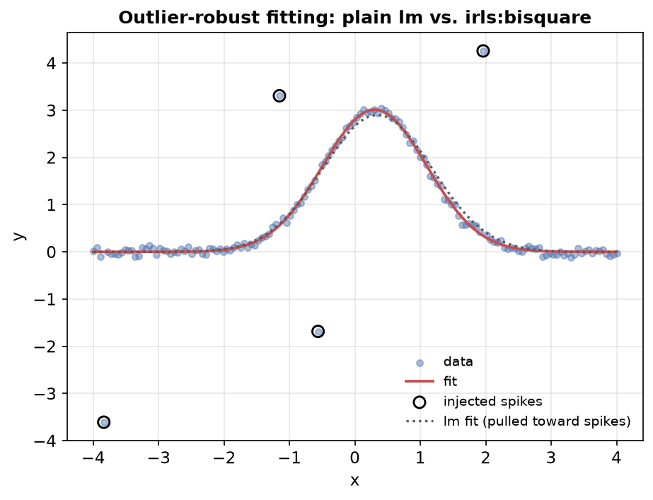
The fixture below is a single seeded peak with a handful of deliberately injected spike outliers — chosen to demonstrate IRLS down-weighting on a known-truth case, not a sweep proving robustness across outlier fraction, magnitude, or real detector-glitch statistics.

Quick example¶

A handful of corrupted or spiked data points — detector glitches, cosmic-ray hits — shouldn't be allowed to drag a plain least-squares fit off the true peak. "irls" / "irls:bisquare" / "irls:cauchy" down-weight points with large residuals automatically instead of treating every point as equally trustworthy.

def synthesize_data() -> tuple[np.ndarray, np.ndarray, np.ndarray]:
    """Synthesize a clean Gaussian peak, then inject a handful of spike outliers.

    Four points (about 2.7% of the 150-point series) get a spike of 2.5-4.0
    in absolute y-units added to their true value -- 0.83-1.33x the true peak
    amplitude of 3.0 -- at random x-positions and random sign, a stand-in for
    detector glitches or cosmic-ray hits rather than ordinary measurement
    noise. Returns ``(x, y, spike_idx)`` so the spikes can be marked on the
    plot.
    """
    rng = np.random.default_rng(21)
    x = np.linspace(-4, 4, 150)
    y_true = AMPLITUDE_TRUE * np.exp(-0.5 * ((x - CENTER_TRUE) / SIGMA_TRUE) ** 2)
    noise = rng.normal(0, 0.06, len(x))
    y = y_true + noise

    n_spikes = 4
    spike_idx = rng.choice(len(x), n_spikes, replace=False)
    spike_magnitude = rng.uniform(2.5, 4.0, n_spikes)
    spike_sign = np.sign(rng.standard_normal(n_spikes))
    y[spike_idx] += spike_magnitude * spike_sign
    return x, y, spike_idx


x, y, spike_idx = synthesize_data()

Four of 150 points (about 2.7%) have a spike of 2.5-4.0 in absolute y-units added to their true value — 0.83-1.33x the true peak amplitude of 3.0 — at random positions and random sign: spikes, not ordinary measurement noise. The same clean-peak graph shape is fit against this spiked data by both solvers below.

def build_graph() -> FitGraph:
    """A single Gaussian peak, amplitude bounded non-negative."""
    return FitGraph(
        nodes=[
            ModelNodeSpec(
                id="peak",
                model_type=ModelType.GAUSSIAN,
                parameters={
                    "amplitude": Parameter(value=2.0, min=0.0),
                    "center": Parameter(value=0.0),
                    "sigma": Parameter(value=0.5, min=1e-3),
                },
            ),
        ],
    )

"lm" sees every residual as equally informative, including the four spikes; "irls:bisquare" re-weights points with large residuals down across its iterations instead.

def fit_both(x: np.ndarray, y: np.ndarray) -> dict[str, FitResult]:
    """Fit the spiked data with plain ``"lm"`` and with ``"irls:bisquare"``."""
    data = MeasurementData(x=x.tolist(), y=y.tolist())
    return {
        "lm": fit(build_graph(), data, FitOptions(solver="lm")),
        "irls:bisquare": fit(build_graph(), data, FitOptions(solver="irls:bisquare")),
    }


results = fit_both(x, y)
lm_result, irls_result = results["lm"], results["irls:bisquare"]

Reporting the recovered amplitude/center error against the known planted ground truth — not just an eyeballed curve — turns "IRLS looks more robust" into a checked number.

def compare(lm_result: FitResult, irls_result: FitResult) -> None:
    """Report recovered center/amplitude error against ground truth, numerically.

    Not just "IRLS looks better on the plot" — the actual absolute error
    against the known planted ``AMPLITUDE_TRUE``/``CENTER_TRUE`` for both
    solvers, so the outlier-robustness claim is a checked number rather than
    an eyeballed curve.
    """
    print(
        f"{'solver':16s} {'amplitude':>10s} {'|err|':>8s} {'center':>9s} {'|err|':>8s}",
    )
    errors: dict[str, tuple[float, float]] = {}
    for name, result in (("lm", lm_result), ("irls:bisquare", irls_result)):
        amp = result.parameters["peak.amplitude"].value
        center = result.parameters["peak.center"].value
        amp_err = abs(amp - AMPLITUDE_TRUE)
        center_err = abs(center - CENTER_TRUE)
        errors[name] = (amp_err, center_err)
        print(f"{name:16s} {amp:10.4f} {amp_err:8.4f} {center:9.4f} {center_err:8.4f}")

    assert lm_result.success
    assert irls_result.success
    lm_amp_err, lm_center_err = errors["lm"]
    irls_amp_err, irls_center_err = errors["irls:bisquare"]
    assert irls_amp_err < lm_amp_err, (
        "irls:bisquare should recover amplitude closer to truth than plain lm "
        "once the spikes are down-weighted"
    )
    assert irls_center_err < lm_center_err, (
        "irls:bisquare should recover center closer to truth than plain lm "
        "once the spikes are down-weighted"
    )


compare(lm_result, irls_result)

Why this works¶

Distinct from everything else in the gallery: this is the only outlier-robustness example. It is real and tested — tests/unit/spectrafit_core/test_irls_weights.py exercises every IRLS weight variant end-to-end against a spiked fit, pinning that each FitOptions.solver string actually reaches its underlying weight function rather than silently falling through to plain LM. Choosing a Solver recommends "irls:bisquare" (Tukey bisquare weights) once "more than roughly 5-10% of points are corrupted" — heavier contamination than plain "irls"'s Huber weights are tuned for.

What just happened¶

Data creation — a clean Gaussian peak (amplitude=3.0, center=0.3) with light noise, then four spike outliers injected at random positions.
Two fits, one graph shape — fit_both() fits the identical spiked data with FitOptions(solver="lm") and FitOptions(solver="irls:bisquare").
"lm" is visibly pulled toward the spikes — its recovered amplitude and center land measurably farther from the planted ground truth than "irls:bisquare"'s, asserted numerically rather than only shown on the plot.
"irls:bisquare" recovers closer to truth — down-weighting the spikes' residuals across iterations keeps the fit anchored to the true peak shape instead of the corrupted points.

Robust Fitting Against Outliers¶

Quick example¶

Why this works¶

What just happened¶

See also¶