spectrafit vs. lmfit: a moderately complex spectrum¶

Synthetic example

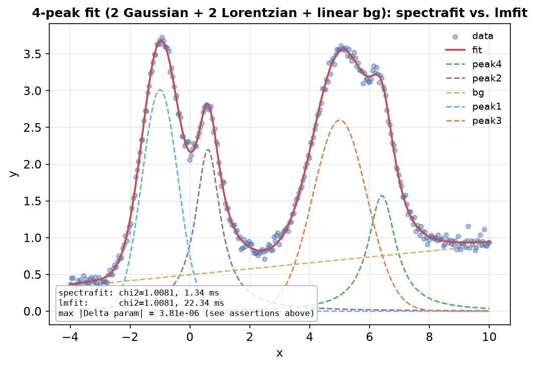
The four-peak spectrum below is built from local numpy formulas with known truth parameters — chosen so both backends' fits can be checked against a known answer, not a sweep proving spectrafit/lmfit agreement across arbitrary real spectra.

Quick example¶

Four overlapping peaks of mixed shape (two Gaussian, two Lorentzian) on a sloped linear background, fitted independently by spectrafit's own fit() and by a hand-built lmfit composite — an external, independently-implemented oracle rather than a second spectrafit solver.

# Per-peak numpy formulas -- same convention as python/oracles/models.py:
# ``amplitude`` is the peak height (not area), Gaussian ``sigma`` is the
# standard deviation, Lorentzian ``sigma`` is the HWHM. These are handed
# straight to ``lmfit.Model`` below, exactly the way
# ``python/oracles/backends/_lmfit.py`` wraps ``PeakModel.evaluate``.
def gaussian(
    x: np.ndarray,
    amplitude: float,
    center: float,
    sigma: float,
) -> np.ndarray:
    """Gaussian peak: ``amplitude`` at ``center``, std-dev ``sigma``."""
    return amplitude * np.exp(-0.5 * ((x - center) / sigma) ** 2)


def lorentzian(
    x: np.ndarray,
    amplitude: float,
    center: float,
    sigma: float,
) -> np.ndarray:
    """Lorentzian peak normalized to ``amplitude`` at ``center`` (HWHM ``sigma``)."""
    return amplitude / (1.0 + ((x - center) / sigma) ** 2)


def linear_bg(x: np.ndarray, slope: float, intercept: float) -> np.ndarray:
    """Linear background ``slope*x + intercept``."""
    return slope * x + intercept

These same raw numpy formulas back both backends' synthetic data below — neither library's own peak-shape convenience function is used, so the comparison starts from identical ground truth rather than two slightly different definitions of "Gaussian".

def synthesize_data() -> tuple[np.ndarray, np.ndarray]:
    """Synthesize the 4-peak + linear-background spectrum (with noise).

    Sums every ``TRUE`` component (2 Gaussian + 2 Lorentzian) plus the
    linear background, then adds Gaussian measurement noise (``sigma=0.06``,
    seeded for reproducibility).
    """
    rng = np.random.default_rng(11)
    x = np.linspace(-4, 10, 320)
    y = (
        gaussian(
            x,
            TRUE["peak1"]["amplitude"],
            TRUE["peak1"]["center"],
            TRUE["peak1"]["sigma"],
        )
        + lorentzian(
            x,
            TRUE["peak2"]["amplitude"],
            TRUE["peak2"]["center"],
            TRUE["peak2"]["sigma"],
        )
        + gaussian(
            x,
            TRUE["peak3"]["amplitude"],
            TRUE["peak3"]["center"],
            TRUE["peak3"]["sigma"],
        )
        + lorentzian(
            x,
            TRUE["peak4"]["amplitude"],
            TRUE["peak4"]["center"],
            TRUE["peak4"]["sigma"],
        )
        + linear_bg(x, BG_TRUE["slope"], BG_TRUE["intercept"])
    )
    noise = rng.normal(0, 0.06, len(x))
    return x, y + noise


x, y = synthesize_data()

Nothing new here — build the graph the same way fitting.md does, just with more nodes (4 peaks + a linear background instead of 1 peak + constant).

def build_graph() -> FitGraph:
    """A 5-node FitGraph: 2 Gaussian + 2 Lorentzian peaks + a linear background."""
    return FitGraph(
        nodes=[
            ModelNodeSpec(
                id="peak1",
                model_type=ModelType.GAUSSIAN,
                parameters={
                    "amplitude": Parameter(value=GUESS["peak1"]["amplitude"], min=0.0),
                    "center": Parameter(value=GUESS["peak1"]["center"]),
                    "sigma": Parameter(value=GUESS["peak1"]["sigma"], min=1e-3),
                },
            ),
            ModelNodeSpec(
                id="peak2",
                model_type=ModelType.LORENTZIAN,
                parameters={
                    "amplitude": Parameter(value=GUESS["peak2"]["amplitude"], min=0.0),
                    "center": Parameter(value=GUESS["peak2"]["center"]),
                    "sigma": Parameter(value=GUESS["peak2"]["sigma"], min=1e-3),
                },
            ),
            ModelNodeSpec(
                id="peak3",
                model_type=ModelType.GAUSSIAN,
                parameters={
                    "amplitude": Parameter(value=GUESS["peak3"]["amplitude"], min=0.0),
                    "center": Parameter(value=GUESS["peak3"]["center"]),
                    "sigma": Parameter(value=GUESS["peak3"]["sigma"], min=1e-3),
                },
            ),
            ModelNodeSpec(
                id="peak4",
                model_type=ModelType.LORENTZIAN,
                parameters={
                    "amplitude": Parameter(value=GUESS["peak4"]["amplitude"], min=0.0),
                    "center": Parameter(value=GUESS["peak4"]["center"]),
                    "sigma": Parameter(value=GUESS["peak4"]["sigma"], min=1e-3),
                },
            ),
            ModelNodeSpec(
                id="bg",
                model_type=ModelType.LINEAR,
                parameters={
                    "slope": Parameter(value=BG_GUESS["slope"]),
                    "intercept": Parameter(value=BG_GUESS["intercept"]),
                },
            ),
        ],
    )

lmfit's own GaussianModel/LorentzianModel normalize by area rather than peak height, which would make a parameter-by-parameter comparison meaningless — so the lmfit side is built by hand from the exact same numpy formulas above, matching spectrafit's peak-height convention exactly.

def build_lmfit_model() -> tuple[lmfit.Model, lmfit.Parameters]:
    """Build the composite lmfit model + params, mirroring LmfitBackend.build()."""
    composite = None
    params = None
    for prefix, fn, _node_id, guess in COMPONENTS:
        m = lmfit.Model(fn, prefix=prefix)
        composite = m if composite is None else composite + m
        pars = m.make_params(**guess)
        if "sigma" in guess:
            pars[f"{prefix}sigma"].set(min=1e-6)
        if "amplitude" in guess:
            pars[f"{prefix}amplitude"].set(min=0.0)
        params = pars if params is None else params.update(pars) or params
    return composite, params

With both backends fit on the same data from the same starting guesses, what's being compared is chi2, wall time, and all 14 fitted parameters side by side.

def run_and_report(
    x: np.ndarray,
    y: np.ndarray,
) -> tuple[FitResult, ModelResult, float, float, float, float]:
    """Fit both backends once each (plus an untimed warm-up), print the report.

    Returns ``(sf_result, lmfit_result, sf_time, lmfit_time, lmfit_chi2,
    max_abs_diff)`` -- everything the assertions step and the ``__main__``
    plotting block need, so neither has to re-run either backend or
    recompute the per-parameter comparison.
    """
    data = MeasurementData(x=x.tolist(), y=y.tolist())

    # Backend 1: spectrafit-core's own fit().
    fit(build_graph(), data)  # warm-up, untimed
    start = time.perf_counter()
    sf_result = fit(build_graph(), data)
    sf_time = time.perf_counter() - start

    # Backend 2: a real lmfit composite model, built by hand exactly the way
    # python/oracles/backends/_lmfit.py's LmfitBackend.build() does: one
    # lmfit.Model(fn, prefix=...) per component, summed with "+", each
    # component's make_params(...) merged into one Parameters object, then
    # composite.fit(y, params, x=x).
    composite, lmfit_params = build_lmfit_model()
    composite.fit(y, lmfit_params, x=x)  # warm-up, untimed
    _, lmfit_params_fresh = build_lmfit_model()
    start = time.perf_counter()
    lmfit_result = composite.fit(y, lmfit_params_fresh, x=x)
    lmfit_time = time.perf_counter() - start

    lmfit_best_fit = np.asarray(lmfit_result.best_fit, dtype=float)
    lmfit_chi2 = float(np.sum((y - lmfit_best_fit) ** 2))

    print(f"{'backend':10s} {'success':8s} {'chi2':>12s} {'wall time':>14s}")
    print(
        f"{'spectrafit':10s} {sf_result.success!s:8s} "
        f"{sf_result.chi2:12.6f} {sf_time * 1e3:11.3f} ms",
    )
    print(
        f"{'lmfit':10s} {lmfit_result.success!s:8s} {lmfit_chi2:12.6f} {lmfit_time * 1e3:11.3f} ms",
    )
    print()

    print(f"{'parameter':16s} {'spectrafit':>12s} {'lmfit':>12s} {'|Delta|':>10s}")
    max_abs_diff = 0.0
    for prefix, _fn, node_id, guess in COMPONENTS:
        for param_name in guess:
            sf_value = sf_result.parameters[f"{node_id}.{param_name}"].value
            lmfit_value = lmfit_result.params[f"{prefix}{param_name}"].value
            diff = abs(sf_value - lmfit_value)
            max_abs_diff = max(max_abs_diff, diff)
            print(
                f"{node_id + '.' + param_name:16s} {sf_value:12.6f} "
                f"{lmfit_value:12.6f} {diff:10.2e}",
            )

    print()
    print(f"Largest |Delta| across all 14 fitted parameters: {max_abs_diff:.2e}")

    return sf_result, lmfit_result, sf_time, lmfit_time, lmfit_chi2, max_abs_diff


sf_result, lmfit_result, sf_time, lmfit_time, lmfit_chi2, max_abs_diff = run_and_report(
    x,
    y,
)

A printed table invites eyeballing "close enough", which can hide a systematic drift a numeric tolerance would catch — so agreement is asserted in code (1e-4 on every parameter and on chi2), not just left for a reader to judge from the table above.

def verify_agreement(
    sf_result: FitResult,
    lmfit_result: ModelResult,
    lmfit_chi2: float,
    max_abs_diff: float,
) -> None:
    """Assert both fits succeeded and agree to within a tight tolerance.

    Both backends should converge to matching parameter values (within
    ``1e-4``) and matching ``chi2`` (within ``1e-4``) on this well-posed
    4-peak + linear-background problem -- in practice both land within
    ``~1e-5`` of each other.
    """
    assert sf_result.success
    assert lmfit_result.success
    assert max_abs_diff < 1e-4, (
        "spectrafit and lmfit should converge to matching parameter values "
        "(within 1e-4) on this well-posed 4-peak + linear-background problem "
        "-- in practice both land within ~1e-5 of each other"
    )
    assert abs(sf_result.chi2 - lmfit_chi2) < 1e-4, (
        "spectrafit and lmfit should converge to matching chi2 on this problem"
    )


verify_agreement(sf_result, lmfit_result, lmfit_chi2, max_abs_diff)

Why this works¶

Why this example exists. Every other script in this gallery cross-checks spectrafit against itself — a different solver (varpro_vs_lm.md), a different parameter surface (shared_params.md), a different dimensionality (3d_fitting.md). This is the first tutorial in this gallery to include lmfit as an external cross-check, not just spectrafit's own alternate solvers. lmfit is a separate, independently-implemented least-squares package — its own Levenberg-Marquardt driver, its own parameter bookkeeping — so agreement with it is a genuinely independent oracle in a way agreement between two spectrafit solvers is not. The project's own benchmark harness (python/oracles/, see Benchmark engine) uses exactly this idea at scale, running spectrafit against lmfit and jax/optimistix across a whole case catalog; this example distills that pattern down to one hand-built, readable script.

Why this scenario. The gallery's other examples are deliberately simple (one or two isolated peaks) so the mechanic being demonstrated stays front-and-center. This one is intentionally more realistic: four overlapping peaks of mixed shape (two Gaussian, two Lorentzian) sitting on a sloped linear background — closer to what a real spectrum (XPS, Raman, UV-Vis, ...) actually looks like than a single clean peak in flat noise.

What just happened¶

Data creation — two Gaussian peaks and two Lorentzian peaks, spaced closely enough to overlap in their wings, on top of a sloped linear background. Both backends are handed the same deliberately-off-true starting guesses (a realistic "eyeballed from the plot" starting point, not the answer key), so the comparison is apples-to-apples.
Backend 1: spectrafit's own fit() — a 5-node FitGraph (4 peaks + one ModelType.LINEAR background node) built by build_graph(), fit with the default solver.
Backend 2: a hand-built lmfit composite model — following the exact pattern used by the project's own lmfit oracle backend (python/oracles/backends/_lmfit.py): one lmfit.Model(fn, prefix=...) per component, summed with +, each component's .make_params(...) merged into one Parameters object, then composite.fit(y, params, x=x). The per-peak numpy formulas (gaussian, lorentzian, linear_bg) use the same convention as python/oracles/models.py: amplitude is the peak height at center (not the integrated area), Gaussian sigma is the standard deviation, and Lorentzian sigma is the half-width at half maximum (HWHM) — a bare hand-rolled lmfit model that matches spectrafit's own convention exactly, rather than lmfit's builtin GaussianModel/LorentzianModel, which normalize by area.
Side-by-side report — a printed table of chi2 and measured wall-clock time per backend, then a second table comparing all 14 fitted parameters (amplitude/center/sigma across 4 peaks, plus the background's slope and intercept) side by side with their absolute difference.
Agreement, asserted not just claimed — the script asserts every fitted parameter agrees between backends to within 1e-4, and chi2 agrees to within 1e-4 too. In practice, on this problem, both land within about 4e-6 of each other — two independently-implemented optimizers converging on the same optimum from the same starting point.

spectrafit vs. lmfit: a moderately complex spectrum¶

Quick example¶

Why this works¶

What just happened¶

See also¶