Single-Dataset Fitting
Synthetic example
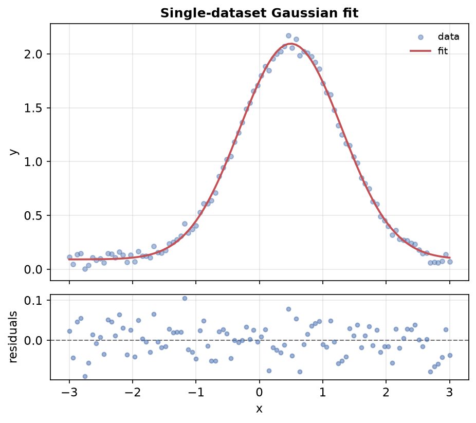
The fixture below is a single seeded Gaussian peak plus constant background with known truth parameters (amplitude 2.0, center 0.5) — chosen so the fit can be checked against a known answer, not a sweep proving this workflow generalizes across peak shapes or noise levels.
Context
When to use this pattern. You have a single measurement (x, y data) and want to fit it with one or more peak models. This is the simplest spectroscopy workflow: create a FitGraph with one or more peak nodes, pass your measured data, and extract the fitted parameters. The result includes the fitted curve, goodness-of-fit metrics (\(R^2\), \(\chi^2\)), and uncertainty estimates.
Quick example
def synthesize_data() -> tuple[np.ndarray, np.ndarray]:
    """Synthesize a single Gaussian peak (amplitude 2.0, center 0.5) in noisy background.

    Adds a 0.1 constant background plus Gaussian measurement noise
    (``sigma=0.05``, seeded for reproducibility).
    """
    rng = np.random.default_rng(42)
    x = np.linspace(-3, 3, 100)
    peak = 2.0 * np.exp(-0.5 * ((x - 0.5) / 0.8) ** 2)
    background = 0.1
    noise = rng.normal(0, 0.05, len(x))
    y = peak + background + noise
    return x, y


x, y = synthesize_data()
We now have noisy (x, y) data with a known ground truth (amplitude 2.0,
center 0.5) — enough to check the fit against later. Next, describe the
model as a graph: one Gaussian peak node plus one constant background node,
each seeded with an initial guess that's deliberately off from the truth.
def build_graph() -> FitGraph:
    """Build a FitGraph: one Gaussian peak + one constant background.

    The ``sigma`` parameter has a lower bound ``min=1e-3`` to prevent the
    optimizer from driving it to zero.
    """
    return FitGraph(
        nodes=[
            ModelNodeSpec(
                id="peak",
                model_type=ModelType.GAUSSIAN,
                parameters={
                    "amplitude": Parameter(value=1.5),
                    "center": Parameter(value=0.0),
                    "sigma": Parameter(value=0.5, min=1e-3),
                },
            ),
            ModelNodeSpec(
                id="bg",
                model_type=ModelType.CONSTANT,
                parameters={
                    "c": Parameter(value=0.0),
                },
            ),
        ],
    )


graph = build_graph()
With data and model in hand, run the solver. fit() dispatches to the
default "lm" (Levenberg-Marquardt) solver, which iterates until the
residuals stop improving.
def run_fit(graph: FitGraph, x: np.ndarray, y: np.ndarray) -> FitResult:
    """Wrap the measurement data and invoke the Levenberg-Marquardt solver.

    ``fit(graph, data)`` iteratively adjusts parameters to minimize the
    residuals until convergence.
    """
    data = MeasurementData(x=x.tolist(), y=y.tolist())
    return fit(graph, data)


result = run_fit(graph, x, y)
The FitResult carries everything needed to judge the fit: whether it
converged, how good it is, and the recovered parameters with uncertainty.
def report_result(result: FitResult) -> None:
    """Print success/goodness-of-fit, fitted parameters, and residual summary.

    Reads ``success`` (did the solver converge), ``r_squared`` and ``chi2``
    (goodness-of-fit), ``parameters`` (value ± stderr per fitted parameter,
    1sigma), and ``residuals`` (observed minus fitted, whose RMS and range
    describe noise level and systematic error).
    """
    print(f"Success: {result.success}")
    print(f"R²: {result.r_squared:.6f}")
    print(f"χ²: {result.chi2:.6f}")
    print()

    for param_name, param in sorted(result.parameters.items()):
        print(f"{param_name:15s} = {param.value:8.4f} ± {param.stderr:8.4f}")
    print()

    residuals = np.array(result.residuals)
    print(f"Residual RMS:   {np.sqrt(np.mean(residuals**2)):.6f}")
    print(f"Residual range: [{np.min(residuals):.6f}, {np.max(residuals):.6f}]")


report_result(result)
What just happened
-
Data creation — we synthesized x, y values (100 points) with a 2.0-amplitude Gaussian centered at 0.5, a 0.1 constant background, and Gaussian noise.
-
Graph definition — we built a
FitGraphwith two nodes:peak: a Gaussian with initial guesses (amplitude=1.5, center=0, sigma=0.5).bg: a constant with initial guess 0.
The
sigmaparameter has a lower boundmin=1e-3to prevent the optimizer from driving it to zero. -
Fit execution —
fit(graph, data)invokes the Levenberg-Marquardt solver (default), which iteratively adjusts parameters to minimize the residuals until convergence. -
Result inspection — we read:
success— True if the solver converged.r_squared— the coefficient of determination (aim for > 0.99 on good data).chi2— the sum of squared residuals.parameters— dict of fitted parameters withvalue(point estimate) andstderr(estimated standard error, \(1\sigma\) — the square root of the covariance diagonal, not a confidence-interval half-width).residuals— the observed minus fitted values; their RMS and range tell you about noise level and systematic errors.
See also
- Related examples:
shared_params.md(tied parameters),multi_dataset.md(joint multi-dataset fits). - Tests:
tests/unit/spectrafit_core/test_fit.py::test_single_gaussian_recovery(noiseless Gaussian),tests/unit/spectrafit_core/test_fit.py::test_components_sum_equals_best_fit(peak + background decomposition). - API docs:
FitGraph,ModelNodeSpec,ModelType,Parameter,MeasurementData,FitResult.