A Wrong Model with a Good \(r^2\)
Real measured data, redistributable under ODbL
This page fits
reproducibility/spectra/eelsdb-fe2o3-l23/DspecTi3wqG.msa, the Fe
\(L_{2,3}\) edge of \(\text{Fe}_2\text{O}_3\), from the
EELS Database. The data is
published under the Open Data Commons Open Database License (ODbL),
which permits redistribution with attribution — so the spectrum ships with
this repository and you can refit it yourself. Credit is due to the
EELS Data Base and to the contributor, Qiang Xu. Cite Ewels P, Sikora T,
Serin V, Ewels CP, Lajaunie L. A Complete Overhaul of the Electron
Energy-Loss Spectroscopy and X-Ray Absorption Spectroscopy Database:
eelsdb.eu. Microscopy and Microanalysis. 2016;22(3):717-724.
doi:10.1017/S1431927616000179.
The ODbL applies to the data; this repository's code stays MIT. Full notice:
that directory's README.md.
Quick example
Every other page in this gallery fits data the model can actually describe. This one deliberately does not, using a real measurement rather than a synthetic fixture, because the effect it demonstrates is a property of real spectra.
def read_msa(path: Path) -> tuple[np.ndarray, np.ndarray]:
    """Read an EMSA/MAS ``.msa`` spectrum into ``(x, y)``.

    The format is a block of ``#KEYWORD : value`` header lines followed by the
    data, terminated by ``#ENDOFDATA``. This file is ``#DATATYPE : XY``, so each
    data row is a comma-separated ``x, y`` pair; skipping every ``#``-prefixed
    line handles the header and the terminator in one rule.
    """
    x: list[float] = []
    y: list[float] = []
    for line in path.read_text(encoding="latin-1").splitlines():
        if not line.strip() or line.startswith("#"):
            continue
        left, _, right = line.partition(",")
        x.append(float(left))
        y.append(float(right))
    return np.asarray(x), np.asarray(y)


def load_l3_window() -> tuple[np.ndarray, np.ndarray]:
    """Load the measured spectrum and cut to the L3 region.

    The window spans the L3 white line at 710.75 eV and the shoulder below it,
    and stops short of the L2 edge near 723 eV so the comparison stays about one
    absorption region rather than the whole spectrum. Intensities are raw
    detector counts, not normalised.
    """
    raw_x, raw_y = read_msa(SPECTRUM)
    lo, hi = WINDOW_EV
    keep = (raw_x >= lo) & (raw_x <= hi)
    return raw_x[keep], raw_y[keep]


x, y = load_l3_window()
The window spans the L3 white line at 710.75 eV and the shoulder below it, stopping short of the L2 edge near 723 eV so the comparison stays about one absorption region. Intensities are raw detector counts, not normalised.
def _peak(index: int, model_type: ModelType, amplitude: float, center: float) -> ModelNodeSpec:
    """One bounded peak component; Voigt gets its extra Lorentzian width."""
    parameters = {
        "amplitude": Parameter(value=amplitude, min=0.0),
        "center": Parameter(value=center, min=float(x.min()), max=float(x.max())),
        "sigma": Parameter(value=1.0, min=0.05, max=8.0),
    }
    if model_type is ModelType.TRUE_VOIGT:
        parameters["gamma"] = Parameter(value=0.5, min=1e-3, max=8.0)
    return ModelNodeSpec(id=f"p{index}", model_type=model_type, parameters=parameters)


def fit_ladder(x: np.ndarray, y: np.ndarray) -> dict[str, FitResult]:
    """Three models of increasing elaboration, fitted to the same window."""
    gaussian, voigt = ModelType.GAUSSIAN, ModelType.TRUE_VOIGT
    peak_height = float(y.max())
    ladder = {
        "1 Gaussian": [_peak(0, gaussian, peak_height, 710.75)],
        "2 Gaussians": [
            _peak(0, gaussian, peak_height, 710.75),
            _peak(1, gaussian, peak_height * 0.3, 708.5),
        ],
        "3 Voigts": [
            _peak(0, voigt, peak_height, 710.75),
            _peak(1, voigt, peak_height * 0.3, 708.5),
            _peak(2, voigt, peak_height * 0.2, 713.5),
        ],
    }
    data = MeasurementData(x=x.tolist(), y=y.tolist())
    return {
        name: fit(FitGraph(nodes=nodes), data, FitOptions(solver="lm"))
        for name, nodes in ladder.items()
    }


results = fit_ladder(x, y)
A run is a maximal stretch of same-signed residuals. Independent noise around a correct model gives about \(2 n_+ n_- / n + 1\) runs; far fewer means the signs arrive in long stretches — the curve sits systematically above the data in one place and below it in another.
def runs_z(residuals: np.ndarray) -> tuple[int, float, float]:
    """Wald-Wolfowitz runs test on the residual signs.

    A *run* is a maximal stretch of same-signed residuals. Residuals that
    are independent noise around a correct model produce about
    ``2*n_pos*n_neg/n + 1`` runs; far fewer means the signs come in long
    stretches, i.e. the curve is systematically above the data in one place
    and below it in another. Returns ``(observed, expected, z)``.

    Caveat, stated because it changes how hard the number may be pushed:
    the test assumes independent residuals. This spectrum is heavily
    oversampled -- 0.05 eV channels against a 0.3 eV instrumental resolution,
    so roughly six channels per resolvable feature -- and genuinely correlated
    measurement noise would also depress the run count. Read a large negative z
    as strong corroboration of what the residual panel already shows, not as a
    calibrated p-value.
    """
    signs = np.sign(residuals)
    signs = signs[signs != 0]
    n = len(signs)
    n_pos = int((signs > 0).sum())
    n_neg = n - n_pos
    observed = int((signs[1:] != signs[:-1]).sum()) + 1
    expected = 2.0 * n_pos * n_neg / n + 1.0
    variance = (expected - 1.0) * (expected - 2.0) / (n - 1.0)
    return observed, expected, (observed - expected) / np.sqrt(variance)


def report(results: dict[str, FitResult]) -> None:
    """Print the ladder, and assert the point it is here to make."""
    print(f"{'model':13s} {'r^2':>9s} {'AIC':>9s} {'runs':>6s} {'expected':>9s} {'z':>7s}")
    stats = {}
    for name, result in results.items():
        observed, expected, z = runs_z(np.array(result.residuals))
        stats[name] = (result.r_squared, result.aic, z)
        print(
            f"{name:13s} {result.r_squared:9.5f} {result.aic:9.1f} "
            f"{observed:6d} {expected:9.1f} {z:7.1f}",
        )

    r2s = [s[0] for s in stats.values()]
    aics = [s[1] for s in stats.values()]
    zs = [s[2] for s in stats.values()]

    # Both scalar scores improve monotonically down the ladder ...
    assert r2s == sorted(r2s), "r^2 should climb at every rung"
    assert aics == sorted(aics, reverse=True), "AIC should fall at every rung"
    # ... while the residuals stay structured at every rung, including the last.
    assert max(zs) < -5.0, "every rung should remain far from random residuals"
    assert results["3 Voigts"].r_squared > 0.95, "the last rung should look excellent"


report(results)
Why this works
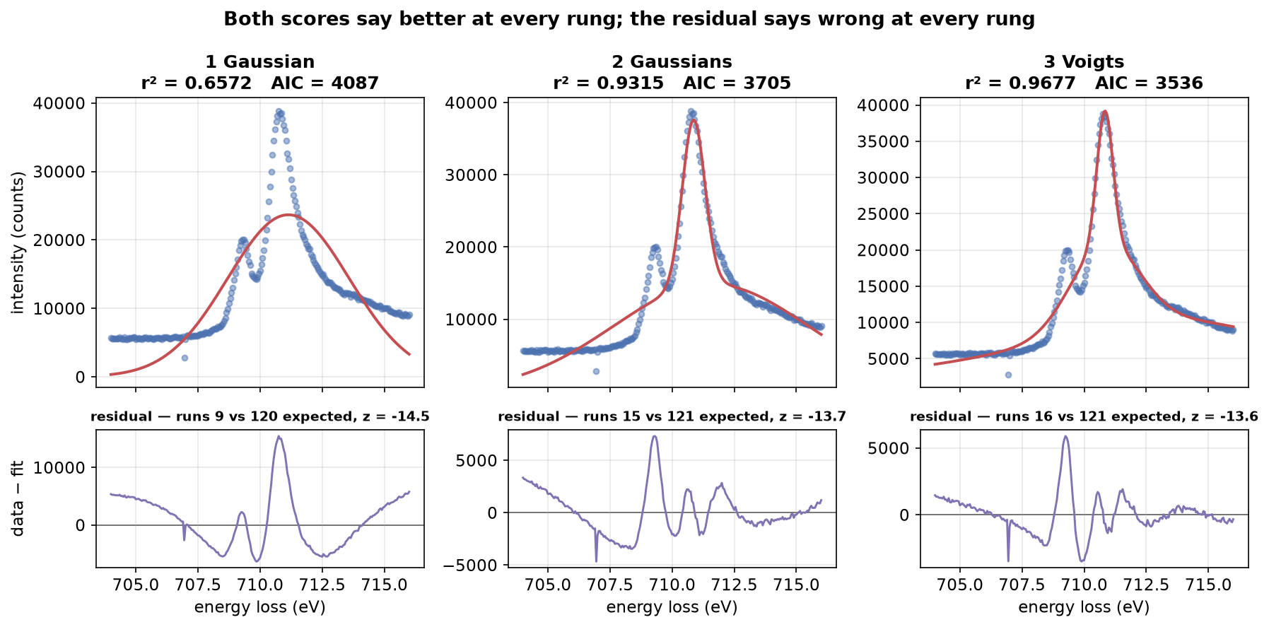
Each other page in this gallery therefore ends with a high \(r^2\) that means what it appears to mean. Three models of the same L3 window, in increasing order of elaboration, are compared here instead. Watch two scalar goodness-of-fit scores and one property of the residual disagree completely:
| model | \(r^2\) | AIC | runs | expected | \(z\) |
|---|---|---|---|---|---|
| 1 Gaussian | 0.65723 | 4087.3 | 9 | 120.4 | \(-14.5\) |
| 2 Gaussians | 0.93153 | 3705.2 | 15 | 120.8 | \(-13.7\) |
| 3 Voigts | 0.96773 | 3535.9 | 16 | 121.5 | \(-13.6\) |
\(r^2\) climbs to 0.97. AIC falls by 551. Both say "better" at every rung. The runs test says "still the wrong model" at every rung, including the last — and unlike \(r^2\), it barely moves.
What just happened
-
One Gaussian (\(r^2 = 0.657\)) — captures the white line and nothing else. The shoulder below it and the decay above are missed entirely and the residual carries both whole. Not a subtle failure; included as the baseline.
-
Two Gaussians (\(r^2 = 0.932\)) — now the shoulder has a component too, and the fit looks convincing at a glance. The residual has shrunk substantially but kept its shape: the same oscillation across the white line, because a Gaussian cannot produce the line's wings.
-
Three Voigts (\(r^2 = 0.968\)) — a defensible model, and by both scalar scores an excellent one. Yet the residual still oscillates through the white line at \(z = -13.6\), statistically indistinguishable from rung 1's \(-14.5\). The remaining structure is real, and there are two independent reasons for it. An Fe L3 edge carries multiplet structure that no small number of independent symmetric components reproduces. And a core-loss edge sits on a decaying background from lower-energy excitations that none of these three models includes at all.
The residual amplitude falls at every rung. The residual shape does not. That distinction is invisible to \(r^2\) and to AIC, both of which reduce the residual to a single number and discard the ordering that carries the evidence.
What the runs test does and does not license
The test assumes independent residuals. This spectrum is heavily oversampled — 0.05 eV channels against a 0.3 eV instrumental resolution, so roughly six channels per resolvable feature — and genuinely correlated measurement noise would also depress the run count. Read a large negative \(z\) as strong corroboration of what the residual panel already shows, not as a calibrated p-value. The claim here is "the residual is not noise", not a significance level.
What to do about it
- Plot the residual. Always. Every conclusion on this page comes from the bottom row of the figure; the top row alone would have been persuasive and wrong.
- Prefer a diagnostic that uses residual order — a runs test, a Durbin-Watson statistic, an autocorrelation — over one that does not. \(r^2\), \(\chi^2_\text{red}\), AIC and BIC are all order-blind.
- Do not fix structure by adding components. Rungs 2 and 3 do exactly that and the structure survives both. A residual that keeps its shape while shrinking is telling you the form is wrong, not that the count is too low.
- Ask what the model is missing, not how many peaks it needs. Here the honest next step is a background term and a multiplet-aware line shape, not a fourth Voigt.
- Let AIC/BIC rank models you already believe, rather than certify that any of them is right. Rung 3 wins the AIC comparison decisively and is still rejected by the residual.
See also
- Related examples:
failed_fit.md(the other way to be misled — a converged fit reportingsuccess=Truewith a negative \(r^2\)),confidence_intervals.md(uncertainties on parameters that assume the model is correct to begin with). - API docs:
FitResult.residuals,FitResult.r_squared,FitResult.aic,FitResult.bic. - Glossary: Glossary — definitions for this page's
project-specific terms (
residual,AIC,BIC).