Escaping Local Minima with the Global Solver
Synthetic example
The fixture below is a single seeded, deliberately bad-start two-peak
problem, chosen to demonstrate the mechanism — not a sweep proving
"global" always escapes a bad local optimum, at any problem size or
starting-guess distance.
Quick example
Initial guesses are poor, or the objective is genuinely multi-modal — two
overlapping peaks with ambiguous or swapped starting positions. "global"
(Differential Evolution + LM refinement, per FitOptions.solver's own
docstring) explores the full parameter space before refining locally, where
a local solver like "lm" would just converge — cleanly, with
success=True — to the wrong answer.
def synthesize_data() -> tuple[np.ndarray, np.ndarray]:
    """Synthesize two well-separated Gaussian peaks (with noise)."""
    rng = np.random.default_rng(4)
    x = np.linspace(-6, 6, 200)
    y_true = PEAK1_TRUE["amplitude"] * np.exp(
        -0.5 * ((x - PEAK1_TRUE["center"]) / PEAK1_TRUE["sigma"]) ** 2,
    ) + PEAK2_TRUE["amplitude"] * np.exp(
        -0.5 * ((x - PEAK2_TRUE["center"]) / PEAK2_TRUE["sigma"]) ** 2,
    )
    noise = rng.normal(0, 0.05, len(x))
    y = y_true + noise
    return x, y


x, y = synthesize_data()
Two well-separated true peaks, but the graph below seeds both nodes'
center at the same wrong location — squarely between the two true peaks,
with no gradient information pointing a local solver toward the correct
split.
def build_graph() -> FitGraph:
    """Two Gaussian nodes, both initial ``center`` guesses seeded at 0.0.

    A deliberately bad start: rather than guessing near either true peak
    (-3.0 and 3.0), both nodes start at the same wrong location, squarely
    between them. A local solver has no gradient information pointing it
    toward the correct two-peak split from here.
    """
    return FitGraph(
        nodes=[
            ModelNodeSpec(
                id="p1",
                model_type=ModelType.GAUSSIAN,
                parameters={
                    "amplitude": Parameter(value=1.0, min=0.0),
                    "center": Parameter(value=0.0, min=-6.0, max=6.0),
                    "sigma": Parameter(value=1.0, min=1e-3),
                },
            ),
            ModelNodeSpec(
                id="p2",
                model_type=ModelType.GAUSSIAN,
                parameters={
                    "amplitude": Parameter(value=1.0, min=0.0),
                    "center": Parameter(value=0.0, min=-6.0, max=6.0),
                    "sigma": Parameter(value=1.0, min=1e-3),
                },
            ),
        ],
    )
The same bad-start graph is fit by both solvers, timed — "global"'s
differential-evolution search is meaningfully slower per call than "lm"'s
single local descent.
def run_solvers(data: MeasurementData) -> dict[str, tuple[FitResult, float]]:
    """Fit the same bad-start graph with ``"lm"`` and ``"global"``, timed.

    Returns ``{"lm": (result, elapsed_s), "global": (result, elapsed_s)}``.
    Single timed calls, not a median-of-many like ``varpro_vs_lm.py`` —
    ``"global"``'s differential-evolution search is meaningfully slower per
    call, and one measurement is enough to show the order-of-magnitude gap
    without materially slowing down gallery regeneration.
    """
    runs: dict[str, tuple[FitResult, float]] = {}
    for solver_name in ("lm", "global"):
        start = time.perf_counter()
        result = fit(build_graph(), data, FitOptions(solver=solver_name))
        elapsed = time.perf_counter() - start
        runs[solver_name] = (result, elapsed)
    return runs


data = MeasurementData(x=x.tolist(), y=y.tolist())
runs = run_solvers(data)
lm_result, lm_time = runs["lm"]
global_result, global_time = runs["global"]
success=True alone can't distinguish "converged to the right answer" from
"converged, confidently, to the wrong one" — chi2/r_squared against the
data is what actually does.
def compare(lm_result: FitResult, global_result: FitResult) -> None:
    """Report chi2/r_squared for both — the concrete "wrong optimum" evidence.

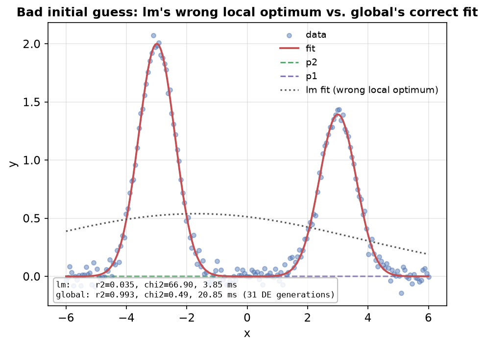
    ``lm``, started with both peaks at the same wrong location, converges
    (``success=True``) to a single broad blob straddling the gap between the
    true peaks rather than resolving two — a textbook local optimum that
    "converged" without being right. ``global`` explores via differential
    evolution first (``n_de_generations`` reports how many generations that
    took) and finds the true two-peak solution.
    """
    print(f"{'solver':8s} {'chi2':>10s} {'r_squared':>10s} {'success':>8s}")
    for name, result in (("lm", lm_result), ("global", global_result)):
        print(
            f"{name:8s} {result.chi2:10.3f} {result.r_squared:10.4f} {result.success!s:>8s}",
        )
    print(f"\nglobal: n_de_generations = {global_result.n_de_generations}")

    assert lm_result.success
    assert global_result.success
    assert global_result.r_squared > 0.98, (
        "global should recover the true two-peak solution on this fixture"
    )
    assert lm_result.r_squared < 0.5, (
        "lm, started with both peaks at the same wrong location, should land "
        "in a visibly wrong local optimum on this fixture"
    )
    assert global_result.chi2 < lm_result.chi2


compare(lm_result, global_result)
Why this works
Distinct from everything else in the gallery: solver="global" does not
appear in any other gallery script (confirmed by grep before writing this
one). It is real and dogfooded internally against synthetic
optimization-landscape test functions in the Rust solver's own test suite,
but this is its first demonstration on a spectroscopy-shaped fit.
What just happened
-
Data creation — two well-separated Gaussian peaks at
center=-3.0andcenter=3.0. -
A deliberately bad start — both graph nodes'
centerinitial guesses are seeded at0.0, the same wrong location. -
"lm"converges to a wrong local optimum —success=True, but a single broad blob straddling the gap between the true peaks (r_squaredwell below the"global"run's, asserted numerically). -
"global"finds the true two-peak solution — differential evolution explores broadly first (n_de_generationsreports how many generations that took) before LM refines locally, landing on the correct split. -
Measured, not general, timing —
"global"took meaningfully longer wall-clock time than"lm"on this one small demo problem; the gap's exact size depends on problem size and hardware, not asserted as a fixed ratio.
See also
- Related examples:
robust_fitting.md(outlier robustness, a different solver-choice axis),bounded_fitting.md(active bounds, a third distinct axis). - Reference: Choosing a Solver.
- API docs:
FitOptions,FitResult.n_de_generations.