VarPro vs. Levenberg-Marquardt
Synthetic example
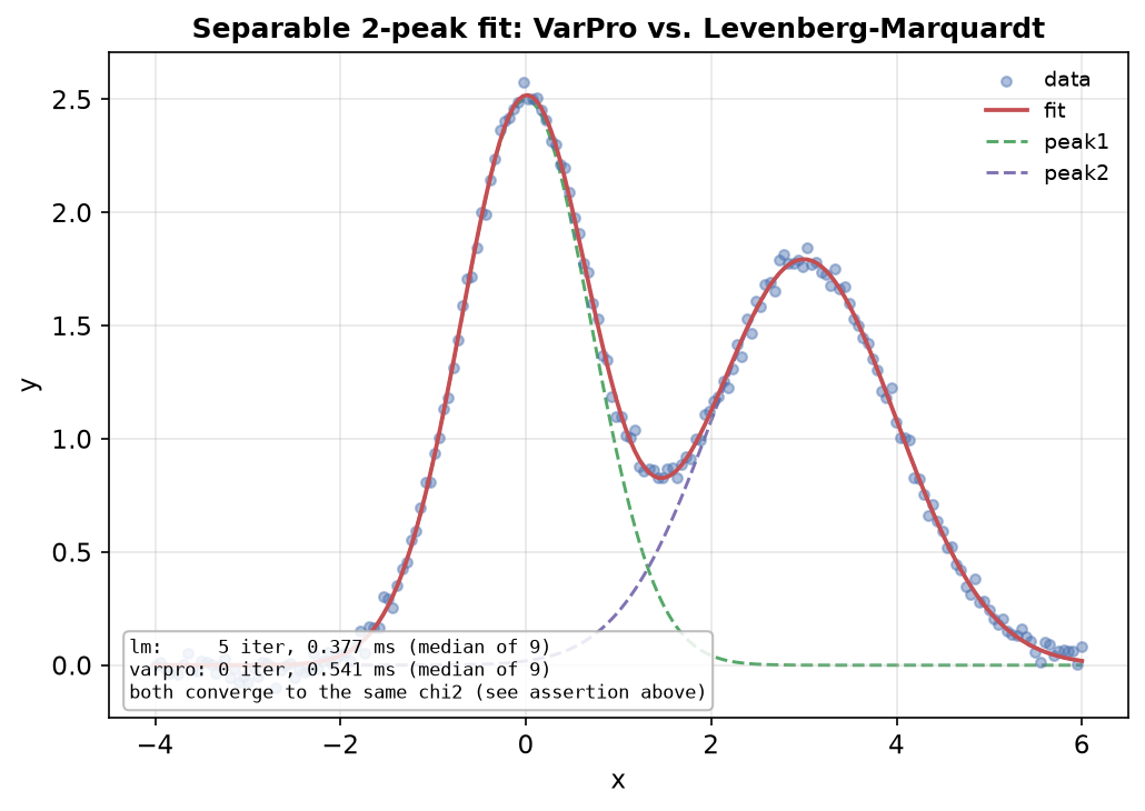
The fixture below is a single seeded, separable two-peak graph with known-truth parameters — chosen to demonstrate that VarPro and LM converge to the identical optimum on a known answer, not a sweep proving this across arbitrary separable-graph shapes.
Context
When to use this pattern. Your model graph is separable — the only
nonlinear parameters are shape parameters like center/sigma, and each
node's amplitude is purely linear, with no tied parameters or bound
constraints on the nonlinear side. This is exactly the shape
FitOptions(solver="auto") itself detects and routes to "varpro" (see
Choosing a Solver). This example fits
the same two-peak graph with both "lm" and "varpro" to show they land on
the identical optimum, from a smaller nonlinear-only parameter space.
Quick example
def synthesize_data() -> tuple[np.ndarray, np.ndarray]:
    """Synthesize two overlapping Gaussians of different width and amplitude.

    No background node — ``amplitude`` is the only linear parameter per
    node, which is what keeps the graph built from this data inside
    VarPro's separability preconditions (see the module docstring).
    """
    rng = np.random.default_rng(7)
    x = np.linspace(-4, 6, 200)
    sigma1_true, sigma2_true = 0.7, 1.0
    center1_true, center2_true = 0.0, 3.0
    peak1_true = 2.5 * np.exp(-0.5 * ((x - center1_true) / sigma1_true) ** 2)
    peak2_true = 1.8 * np.exp(-0.5 * ((x - center2_true) / sigma2_true) ** 2)
    noise = rng.normal(0, 0.04, len(x))
    y = peak1_true + peak2_true + noise
    return x, y


x, y = synthesize_data()
Build a graph over this data with no background node, no bounds, and no
tied parameters — each peak's only linear parameter is amplitude; center
and sigma are nonlinear. That keeps the graph separable, which is
exactly the precondition VarPro needs.
def build_graph() -> FitGraph:
    """A fresh, unbounded, untied FitGraph — VarPro's preconditions hold."""
    return FitGraph(
        nodes=[
            ModelNodeSpec(
                id="peak1",
                model_type=ModelType.GAUSSIAN,
                parameters={
                    "amplitude": Parameter(value=2.0),
                    "center": Parameter(value=0.3),
                    "sigma": Parameter(value=0.5),
                },
            ),
            ModelNodeSpec(
                id="peak2",
                model_type=ModelType.GAUSSIAN,
                parameters={
                    "amplitude": Parameter(value=1.5),
                    "center": Parameter(value=2.7),
                    "sigma": Parameter(value=0.8),
                },
            ),
        ],
    )
fit() is called twice, once per solver, each time on a fresh FitGraph
from build_graph() rather than a reused object — that rules out any doubt
about shared mutable state biasing one solver's starting point against the
other's.
def run_solvers(
    data: MeasurementData,
    n_reps: int = 9,
) -> dict[str, tuple[FitResult, float]]:
    """Fit ``build_graph()`` with both solvers, print the side-by-side report.

    A fresh ``FitGraph`` is built per call (cheap, and avoids any doubt about
    shared mutable state). One untimed warm-up call per solver first
    (import/JIT-style first-call overhead is not representative of
    steady-state solver cost), then the median of ``n_reps`` timed reps.

    Returns ``{"lm": (result, median_time), "varpro": (result, median_time)}``.
    """
    runs: dict[str, tuple[FitResult, float]] = {}
    for solver_name in ("lm", "varpro"):
        result = fit(
            build_graph(),
            data,
            FitOptions(solver=solver_name),
        )  # warm-up, untimed
        times: list[float] = []
        for _ in range(n_reps):
            graph = build_graph()
            start = time.perf_counter()
            result = fit(graph, data, FitOptions(solver=solver_name))
            times.append(time.perf_counter() - start)
        median_time = sorted(times)[len(times) // 2]
        runs[solver_name] = (result, median_time)

    print(
        f"{'solver':8s} {'success':8s} {'n_iter':7s} {'chi2':>12s} {'median wall time':>18s}",
    )
    for name, (result, elapsed) in runs.items():
        print(
            f"{name:8s} {result.success!s:8s} {result.n_iter:7d} "
            f"{result.chi2:12.6f} {elapsed * 1e3:15.3f} ms",
        )
    return runs


# Prepare measurement data (shared across both solver runs).
data = MeasurementData(x=x.tolist(), y=y.tolist())
N_REPS = 9
runs = run_solvers(data, N_REPS)
lm_result, lm_time = runs["lm"]
varpro_result, varpro_time = runs["varpro"]
The two solvers take different optimization paths (six free parameters for
lm, four for varpro, with the two amplitudes solved analytically), so
exact bit-for-bit equality isn't the right bar — a 1e-4 tolerance on
chi2 is what actually distinguishes "converged to the same optimum" from
"drifted to a different one".
def verify_agreement(lm_result: FitResult, varpro_result: FitResult) -> None:
    """Print per-parameter deltas, then assert both solvers agree.

    This is the actual guaranteed property: VarPro is not a different
    model, just a different (smaller) parameter space to search. ``chi2``
    is asserted to match within ``1e-4``; every fitted parameter agrees to
    within ``1e-7`` in practice (see the printed deltas below).
    """
    print()
    print("Fitted parameters agree between solvers to within:")
    for node, param in (
        ("peak1", "amplitude"),
        ("peak1", "center"),
        ("peak1", "sigma"),
        ("peak2", "amplitude"),
        ("peak2", "center"),
        ("peak2", "sigma"),
    ):
        key = f"{node}.{param}"
        diff = abs(
            lm_result.parameters[key].value - varpro_result.parameters[key].value,
        )
        print(f"  {key:18s} Delta = {diff:.2e}")

    assert lm_result.success
    assert varpro_result.success
    assert abs(lm_result.chi2 - varpro_result.chi2) < 1e-4, (
        "lm and varpro should converge to the same optimum on this separable problem"
    )


verify_agreement(lm_result, varpro_result)
What just happened
-
Data creation — two overlapping Gaussian peaks, no background node. Each peak's only linear parameter is its
amplitude;centerandsigmaare the nonlinear shape parameters VarPro's outer optimizer works over. -
Two solver runs, same graph shape —
run_solvers()callsfit()once withFitOptions(solver="lm")and once withFitOptions(solver="varpro"), on a freshFitGraph(frombuild_graph()) each time."lm"optimizes all six free parameters together (2 peaks × 3 params);"varpro"optimizes only the four nonlinear ones (center,sigmaper peak) and solves the two amplitudes analytically at every step. -
Same optimum, different path —
verify_agreement()assertschi2matches between solvers to1e-4, and every fitted parameter agrees to within1e-7in practice. This is the actual guaranteed property: VarPro is not a different model, just a different (smaller) parameter space to search. -
Measured wall-clock time, honestly scoped —
run_solvers()reports the median of 9 timed reps per solver (after an untimed warm-up call) and plots both numbers without declaring a "winner". Whether VarPro or LM is faster in absolute terms depends on problem size, peak count, and hardware — on this small two-peak demo the two are comparable. The project's own aggregate speed comparison across its full benchmark case catalog lives on the Performance page, not in this gallery script.
See also
- Related examples:
shared_params.md(tied parameters — not supported under"varpro"),confidence_intervals.md(uncertainty reporting). - Reference: Choosing a Solver, Rust ↔ Python binding audit.
- API docs:
FitOptions,FitGraph,ModelNodeSpec,fit. - Glossary: Glossary — definitions for this page's
project-specific terms (
VarPro,tied parameters,LM).