Bounded Fitting with an Active-Bounds Solver
Synthetic example
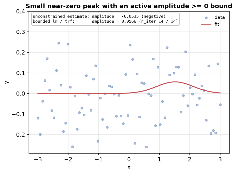
The fixture below is a single seeded, deliberately noise-floor-adjacent peak, chosen to make an unconstrained fit plausibly land at a negative amplitude — not a sweep that proves this happens generally, at any noise level or amplitude.
Quick example
A physical bound — amplitude \(\geq 0\), a mixing fraction \(\in [0, 1]\) — is likely to be active, not just a loose safety floor that never actually binds.
def synthesize_data() -> tuple[np.ndarray, np.ndarray]:
    """Synthesize a small, near-zero-amplitude Gaussian peak with real noise.

    ``AMPLITUDE_TRUE = 0.06`` against a noise standard deviation of ``0.15``
    is deliberately close to the noise floor — small enough that an
    *unconstrained* fit of this data plausibly lands at a negative
    amplitude (see ``build_graph``'s unbounded reference below), which is
    physically meaningless for a peak amplitude.
    """
    rng = np.random.default_rng(5)
    x = np.linspace(-3, 3, 80)
    y_true = AMPLITUDE_TRUE * np.exp(-0.5 * ((x - CENTER_TRUE) / SIGMA_TRUE) ** 2)
    noise = rng.normal(0, 0.15, len(x))
    y = y_true + noise
    return x, y


x, y = synthesize_data()
AMPLITUDE_TRUE = 0.06 against a noise standard deviation of 0.15 sits
close enough to the noise floor that an unconstrained fit of this data
plausibly estimates a negative amplitude — physically meaningless for a
peak. build_graph accepts the bound to apply so the same shape can build
both the unconstrained reference graph and the bounded one.
def build_graph(*, amplitude_min: float) -> FitGraph:
    """One Gaussian peak; ``sigma`` fixed at truth, ``amplitude``/``center`` free.

    ``amplitude_min=0.0`` is the physical bound under test; ``amplitude_min
    = -inf`` builds the unconstrained reference graph used below to show
    what the bound is actually ruling out.
    """
    return FitGraph(
        nodes=[
            ModelNodeSpec(
                id="peak",
                model_type=ModelType.GAUSSIAN,
                parameters={
                    "amplitude": Parameter(value=0.05, min=amplitude_min),
                    "center": Parameter(value=0.2),
                    "sigma": Parameter(value=SIGMA_TRUE, vary=False),
                },
            ),
        ],
    )
Three fits against the identical data: the unconstrained reference (to see
what the bound is actually ruling out), then the bounded problem solved by
both "lm" and "trf".
def fit_all(x: np.ndarray, y: np.ndarray) -> dict[str, FitResult]:
    """Fit the unbounded reference once, then the bounded problem with both solvers."""
    data = MeasurementData(x=x.tolist(), y=y.tolist())
    return {
        "unbounded": fit(build_graph(amplitude_min=float("-inf")), data),
        "lm": fit(build_graph(amplitude_min=0.0), data, FitOptions(solver="lm")),
        "trf": fit(build_graph(amplitude_min=0.0), data, FitOptions(solver="trf")),
    }


results = fit_all(x, y)
unbounded_result, lm_result, trf_result = (
    results["unbounded"],
    results["lm"],
    results["trf"],
)
The unconstrained amplitude going negative is the concrete evidence for why
the bound matters; both bounded solvers are then checked against
min=0 directly rather than trusted by eye.
def compare(
    unbounded_result: FitResult,
    lm_result: FitResult,
    trf_result: FitResult,
) -> None:
    """Report the unbounded amplitude, then both bounded solvers' compliance.

    The unbounded fit's amplitude going negative is exactly the physically
    implausible result the ``min=0`` bound rules out. Both bounded solvers
    are asserted to respect that bound: on this small problem they in fact
    converge to numerically identical iterates (``n_iter`` and the final
    amplitude match) — this codebase's reflective-bounds projection
    (``crates/spectrafit-solver/src/lm_problem.rs``) is shared by every
    LM-family solver, so ``"trf"``'s Coleman–Li step scaling changes *how*
    the optimizer approaches an active bound rather than *whether* it ends
    up inside it. The scaling matters more on problems where a bound stays
    persistently and severely active across many iterations than it does on
    this small demo — this script reports what is actually measured here,
    not a general performance claim.
    """
    unbounded_amp = unbounded_result.parameters["peak.amplitude"].value
    print(f"unconstrained amplitude estimate: {unbounded_amp:.4f} (no min=0 bound)")
    print()
    print(f"{'solver':8s} {'amplitude':>10s} {'n_iter':>7s} {'success':>8s}")
    for name, result in (("lm", lm_result), ("trf", trf_result)):
        amp = result.parameters["peak.amplitude"].value
        print(f"{name:8s} {amp:10.6f} {result.n_iter:7d} {result.success!s:>8s}")

    assert unbounded_result.success
    assert unbounded_amp < 0.0, (
        "this fixture is chosen so the unconstrained amplitude estimate is "
        "negative, motivating the min=0 bound"
    )
    assert lm_result.success
    assert trf_result.success
    bound_tolerance = 1e-9
    assert lm_result.parameters["peak.amplitude"].value >= -bound_tolerance
    assert trf_result.parameters["peak.amplitude"].value >= -bound_tolerance


compare(unbounded_result, lm_result, trf_result)
Why this works
Choosing a Solver recommends "trf"
(Trust Region Reflective) whenever "bounds are frequently active": it adds
Coleman–Li bound scaling that shrinks trust-region steps as a parameter
approaches an active bound. Every LM-family solver in this codebase
(including plain "lm") already shares a reflective-bounds projection, so
"lm" alone never violates [min, max] — "trf" changes how the
optimizer approaches the wall, not whether the final result respects it.
Distinct from varpro_vs_lm.md: that comparison is on an unconstrained
separable problem. This is solver choice under active bound constraints.
What just happened
-
Data creation — a small Gaussian peak (
amplitude=0.06) against comparatively large noise (\(\sigma=0.15\)), synthesized so an unconstrained fit plausibly lands negative. -
Three fits, one graph shape — the unconstrained reference (
amplitude_min=-inf) is fit first, then the bounded problem (amplitude_min=0.0) is fit with both"lm"and"trf". -
The bound is the point — the unconstrained fit's negative amplitude is exactly what
min=0rules out; both bounded solvers are asserted to land inside[0, inf). -
On this small problem,
"lm"and"trf"converge identically — samen_iter, same final amplitude, measured directly rather than assumed. This codebase's reflective-bounds projection is shared by every LM-family solver; Coleman–Li scaling changes the per-iteration step shape near an active bound, which matters more on problems where a bound stays persistently and severely active across many iterations than it does here. This script reports what is actually measured on this fixture, not a general performance claim.
See also
- Related examples:
varpro_vs_lm.md(solver comparison on an unconstrained problem),robust_fitting.md(a different solver-choice axis: outlier robustness, not bounds). - Reference: Choosing a Solver.
- API docs:
FitOptions,Parameter.