Tutorials
Gallery
Runnable, annotated examples — from a single peak to a genuinely 3-D joint fit. Each thumbnail below is generated fresh from the actual checked-in script, not a hand-made screenshot.
A visual index of the runnable examples under docs/tutorials/gallery/. Each
thumbnail is generated by the gallery script of the same name (regenerated by
docs/tutorials/gallery/_render.py, wired into poe docs_build) — click
through to the full tutorial page for the annotated code and the "what just
happened" walkthrough.
Starting
The core mechanics — one concept per example, spectrafit-core's own solvers and features only.
-
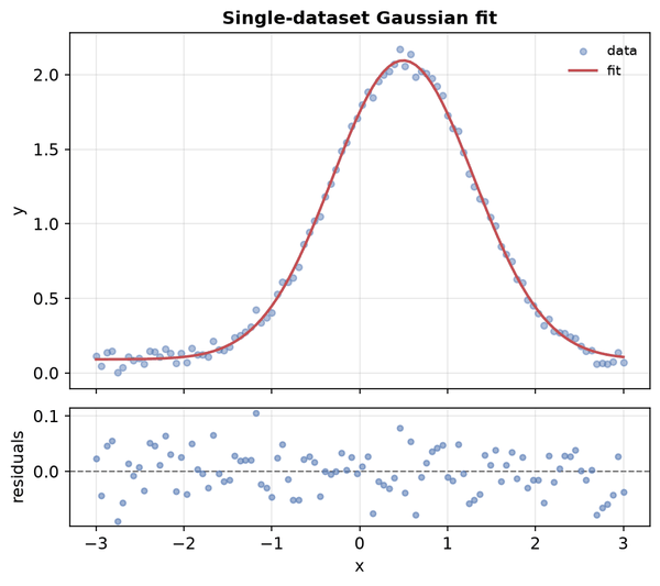
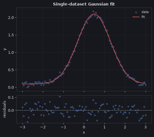
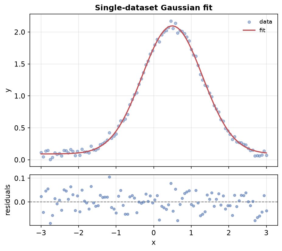
A single Gaussian peak plus constant background, fitted from noisy data with a residuals subplot.
-
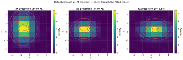
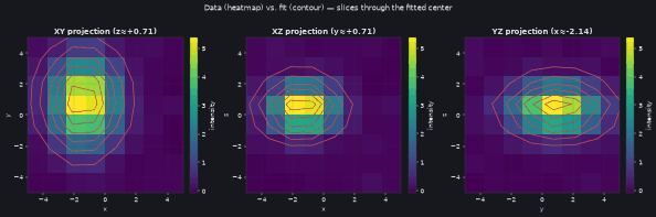
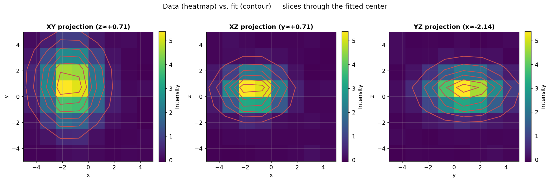
A genuinely 3-D Gaussian recovered in one joint solve, viewed through three fixed-axis slice projections.
-
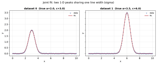
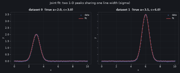
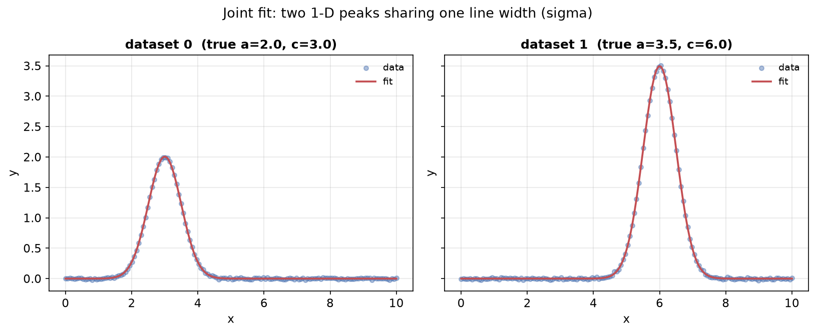
Multi-Dataset Joint Fitting — 1-D
Two 1-D peaks at different positions and amplitudes, fitted jointly with one shared line width.
-
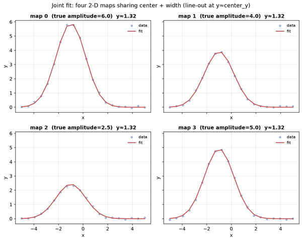
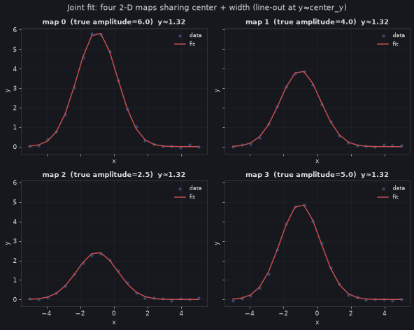
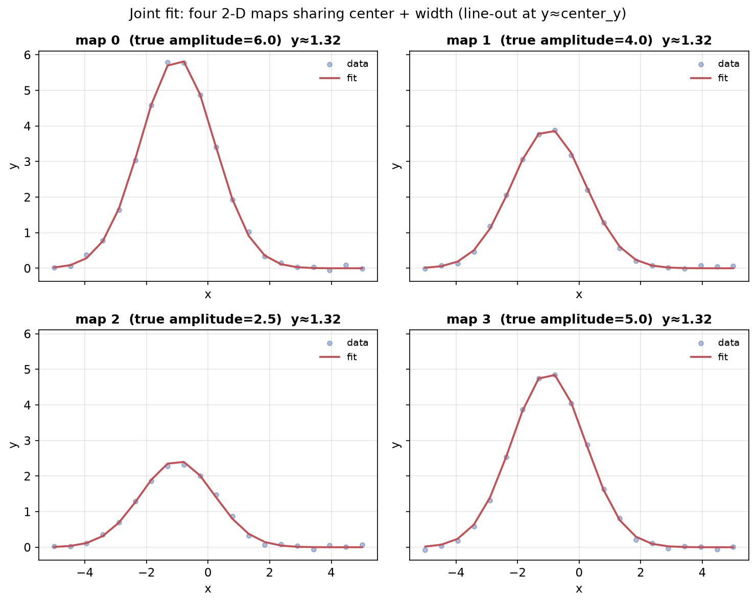
Multi-Dataset Joint Fitting — 2-D
Four 2-D maps differing only in amplitude, fitted jointly with a shared peak center and width.
-
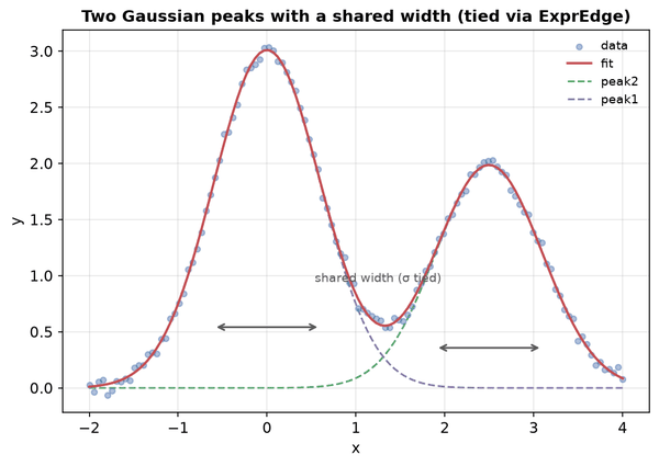
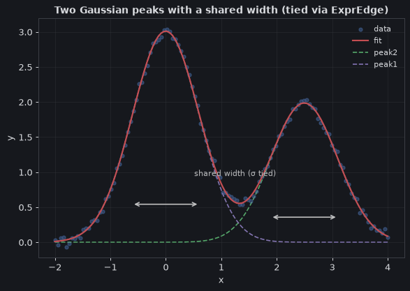
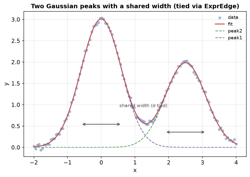
Two overlapping peaks tied to an identical line width via an
ExprEdge, with the shared width annotated on the plot. -
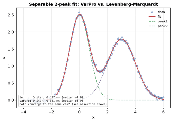
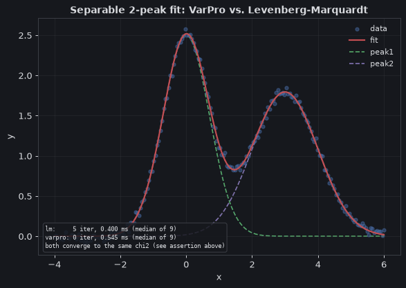
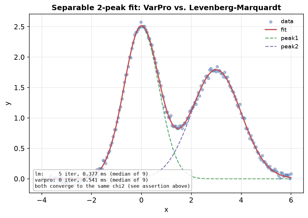
VarPro vs. Levenberg-Marquardt
The same separable two-peak fit solved by both
"varpro"and"lm", converging to the identical optimum from a smaller nonlinear-only parameter space. -
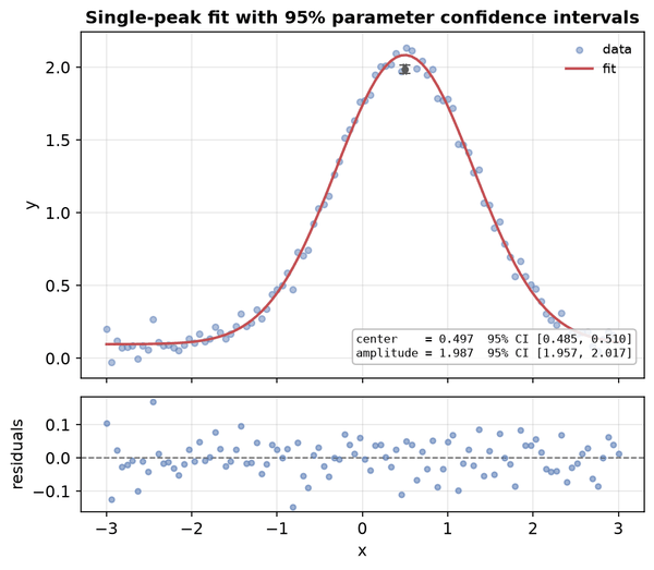
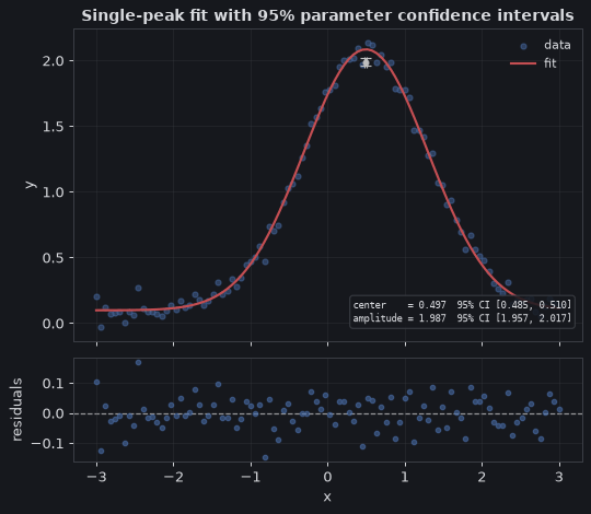
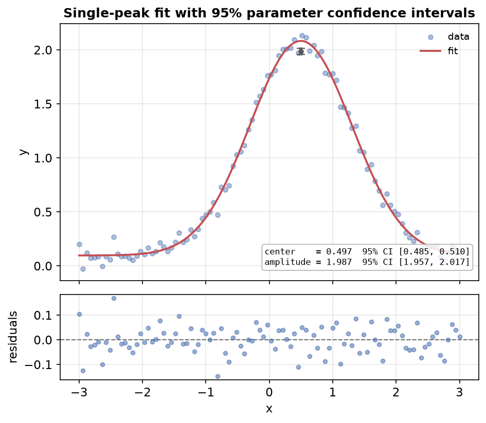
Parameter Confidence Intervals
Turning each fitted parameter's
stderrinto a 95% confidence interval, annotated directly on the plot. -
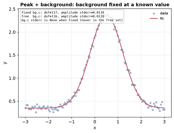
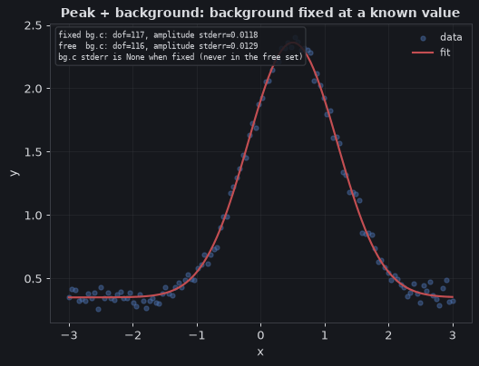
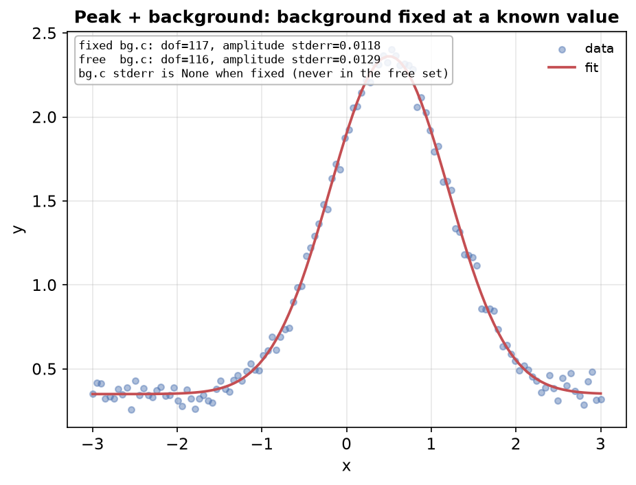
Holding a background level fixed at a value known from an independent measurement, instead of fitting it.
-
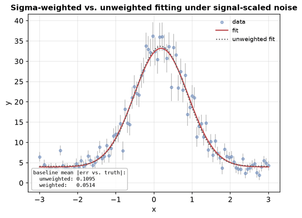
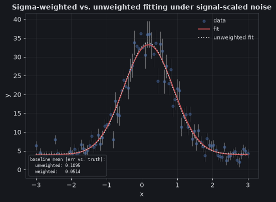
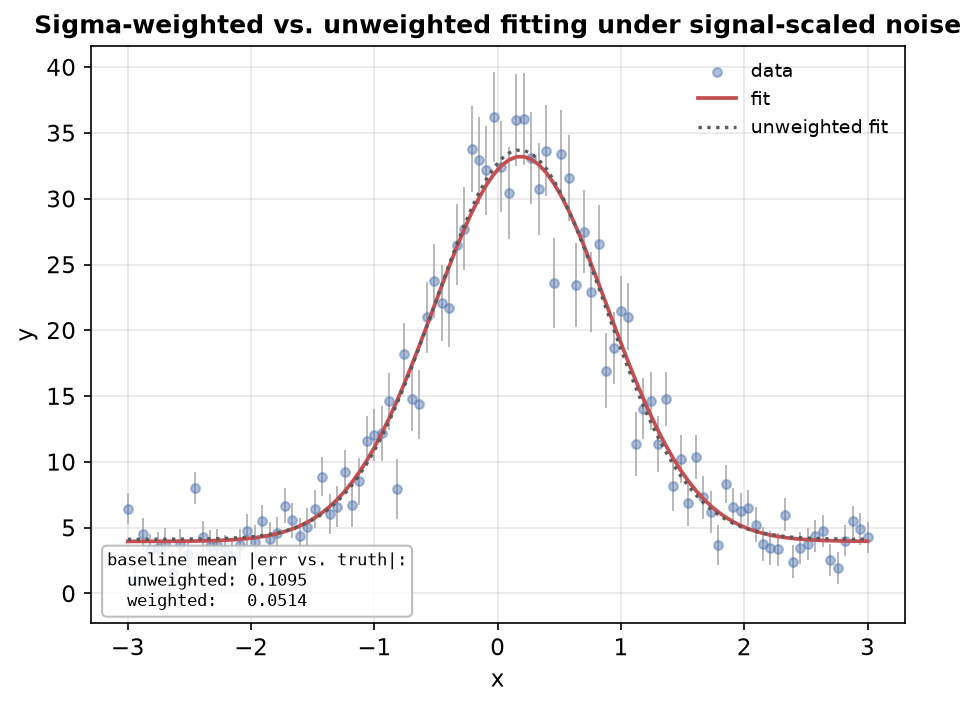
Passing known per-point uncertainty as
sigmaso the fit weights points by their actual reliability instead of treating every point as equally trustworthy.
Solver behavior
Solver-choice demonstrations — the same spectrafit-core solvers from a different angle, where the "right" answer depends on what the data or the constraints actually look like, not just which solver runs fastest.
-
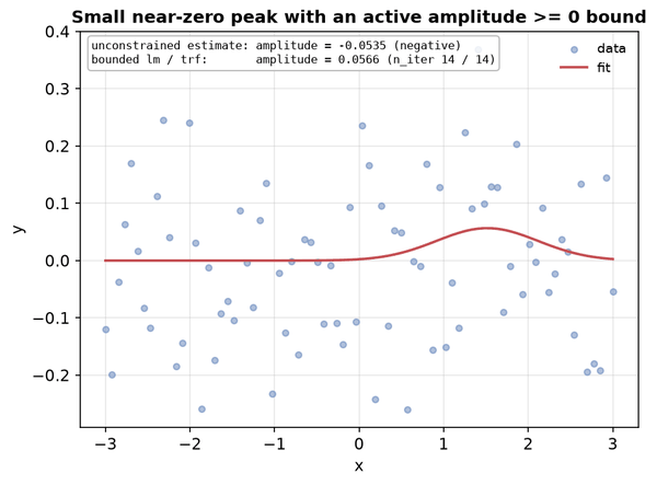
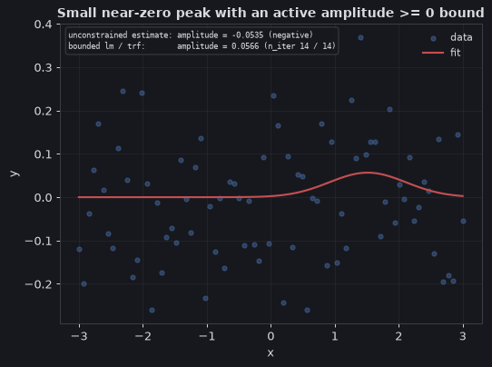
Bounded Fitting with an Active-Bounds Solver
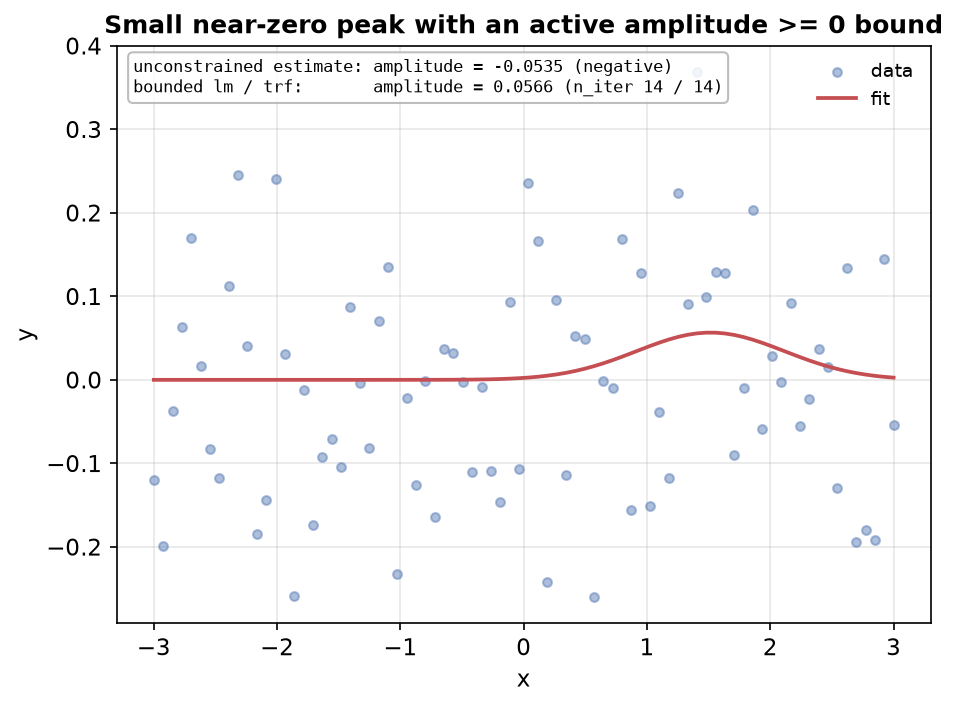
A likely-active physical bound (amplitude ≥ 0) where
"trf"adds Coleman–Li step scaling near the boundary that plain"lm"lacks, though both remain bound-compliant here. -
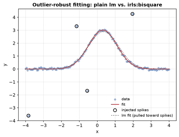
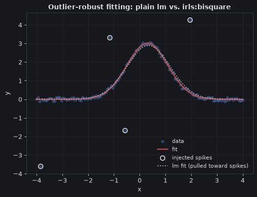
Robust Fitting Against Outliers
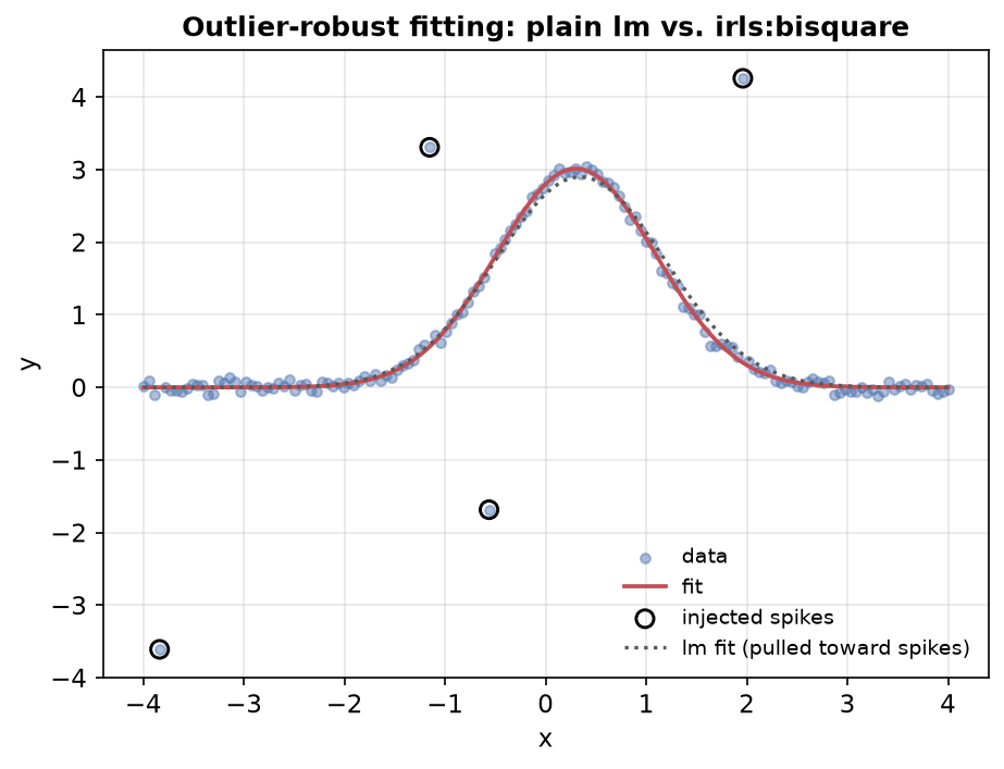
A handful of corrupted spike points down-weighted automatically by
"irls:bisquare", instead of dragging a plain least-squares fit off the true peak. -
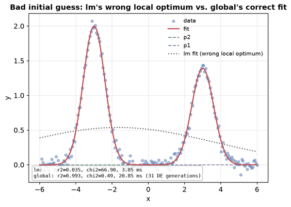
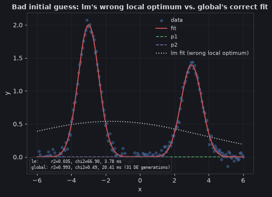
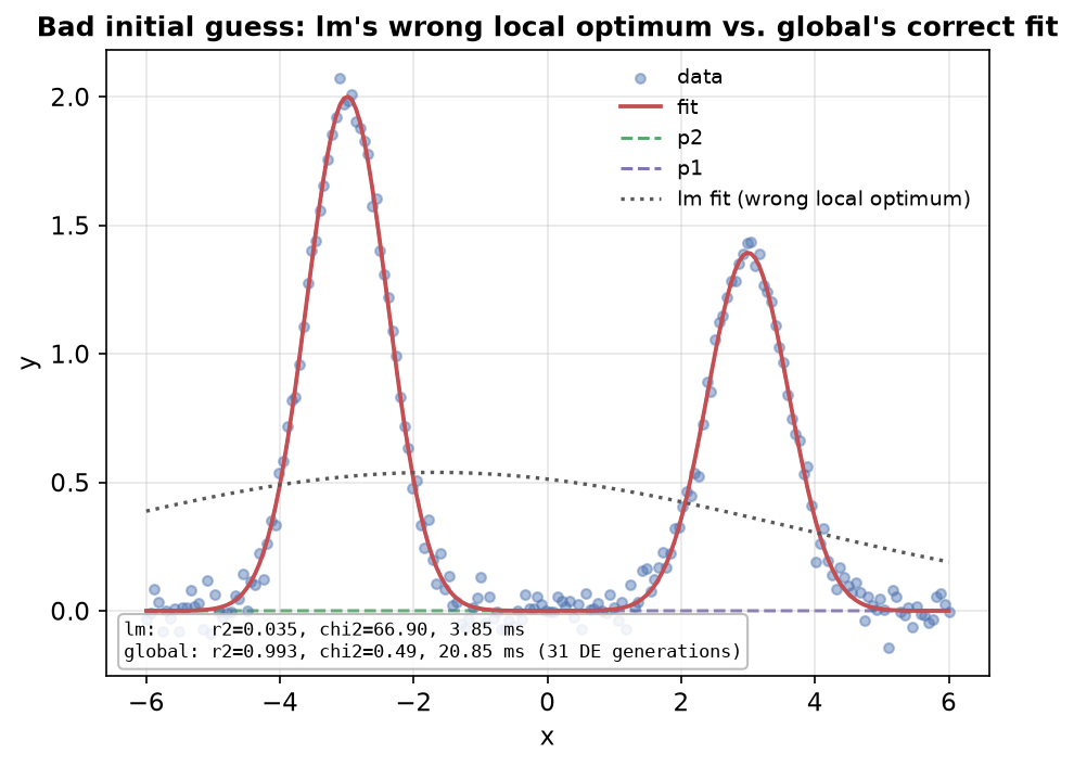
Escaping Local Minima with the Global Solver
A deliberately bad initial guess where
"global"explores broadly before a local solver would just get stuck. -
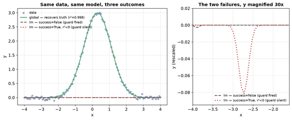
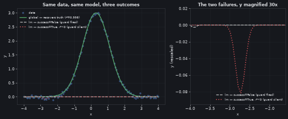
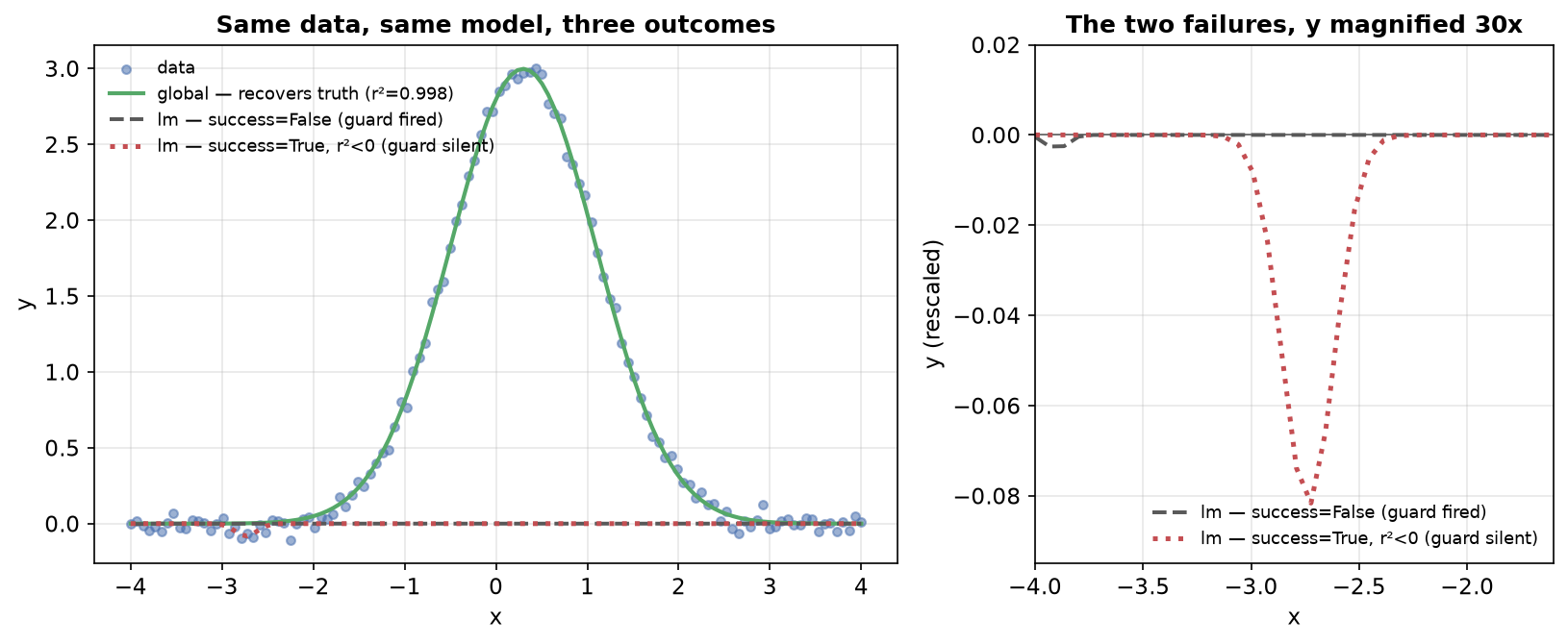
One fit reports
success=Falseand names the reason; another reportssuccess=Truewith a negative \(r^2\). The only difference is a 1% amplitude threshold. -
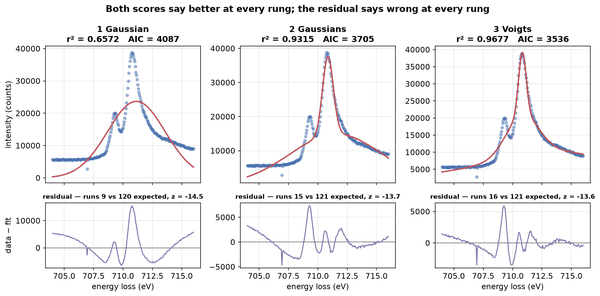
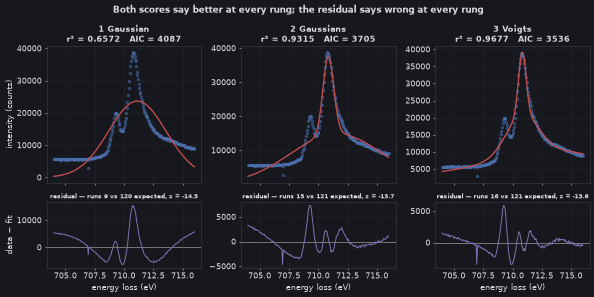
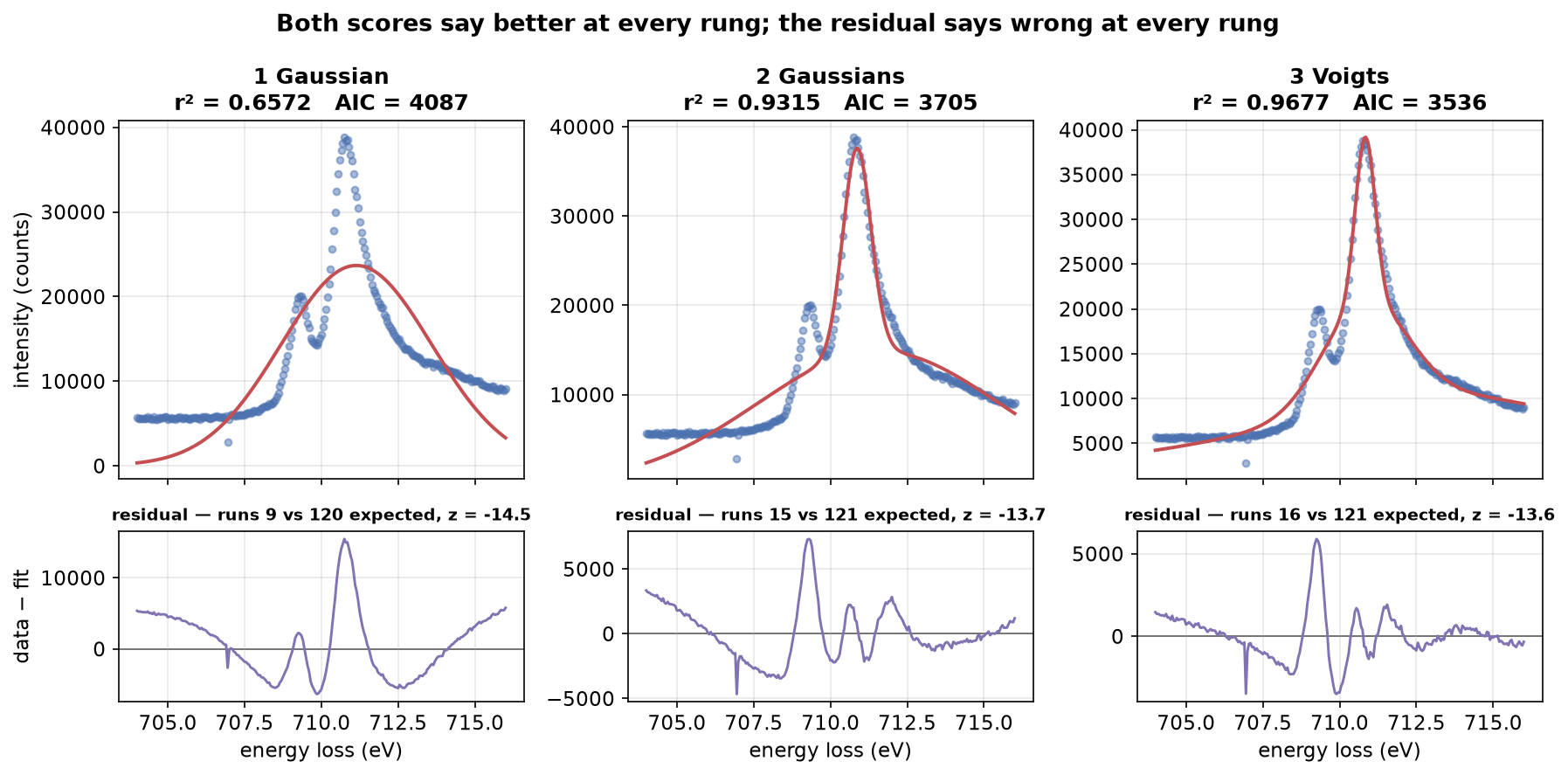
A Wrong Model with a Good \(r^2\)
On real measured data, \(r^2\) climbs to 0.99 and AIC falls by 300 while the residual stays systematically structured at every step.
Advanced
An external, independently-implemented cross-check: lmfit as an oracle, not just spectrafit-core's own alternate solvers — the same idea the project's own benchmark harness runs at scale, distilled into one readable script.
-
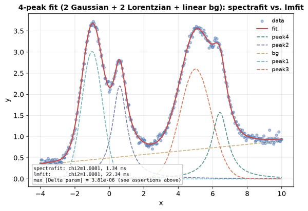
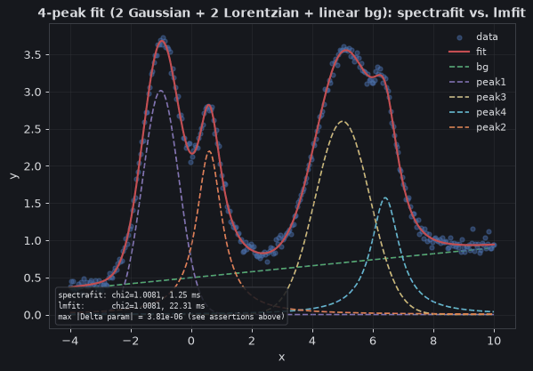
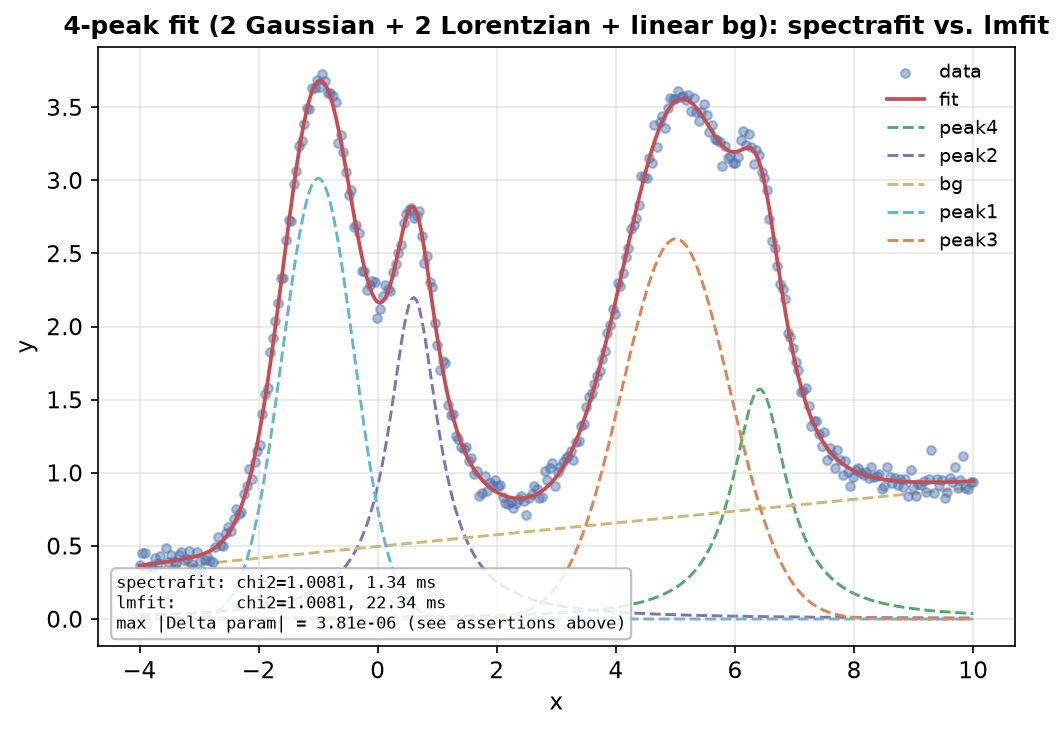
spectrafit vs. lmfit — a moderately complex spectrum
Four overlapping peaks of mixed shape on a sloped background, fitted independently by spectrafit-core and a hand-built lmfit composite — agreeing to within
4e-6.
Extra
The genuinely messy case: more peaks, mixed lineshapes, and a physically-motivated tied parameter — where "do the two independent optimizers actually agree" stops being a given.
-
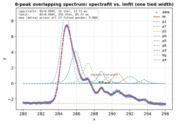
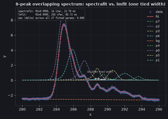
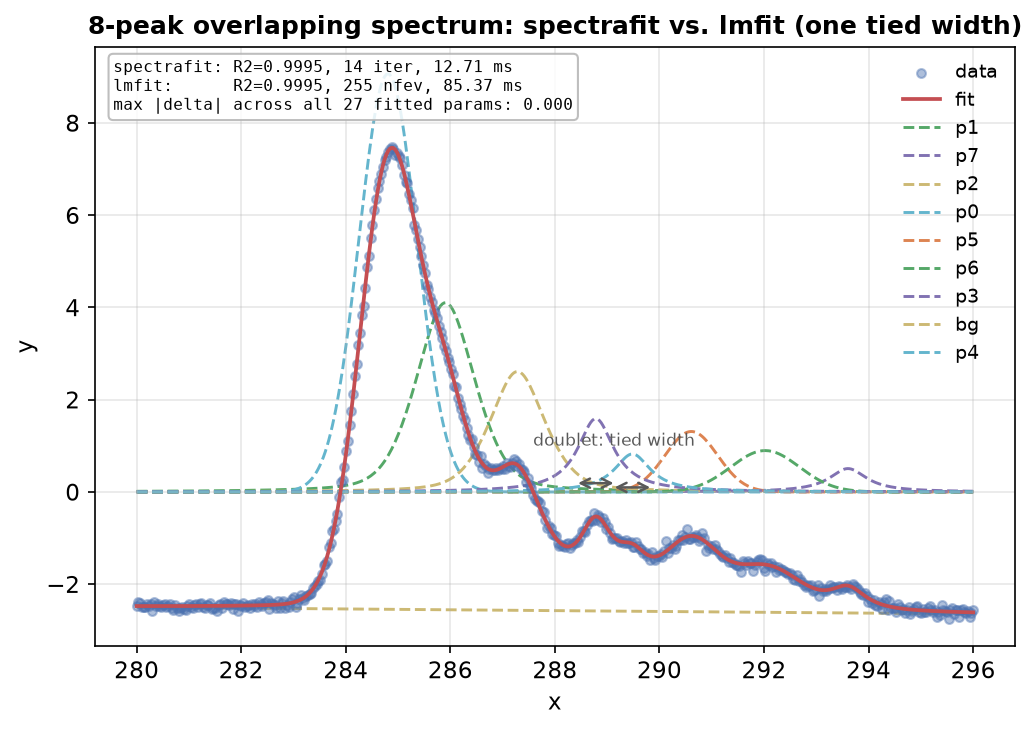
spectrafit vs. lmfit — a complex, 8-peak spectrum
An XPS-style, 8-peak, three-lineshape spectrum with a tied spin-orbit doublet linewidth — spectrafit and lmfit converge to matching \(R^2\) and a loose per-parameter tolerance, honestly reported rather than overclaimed.