Multi-Dataset Joint Fitting¶

Scope of these examples

All examples below are synthetic and illustrative: each uses a single seeded geometry (one model type, one grid size, one noise level, one random seed) chosen to demonstrate the mechanism, not to characterise accuracy across problem sizes, model families, or noise regimes. They show that the joint solve runs and that the shared-parameter ties are enforced within a solve. They are not measured data and are not a sweep that proves general accuracy.

You have N related spectra that share one identical model and want to solve them jointly instead of independently — shared parameters end up constrained by all the data at once, rather than just the one dataset they happen to sit in.

1-D example: local peaks with a shared line width¶

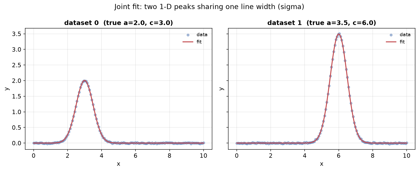
Two Gaussian peaks are recorded at different positions and amplitudes, but the instrument's line-broadening function is known to be identical across measurements (shared sigma). We fit both datasets jointly and recover the per-dataset amplitude and center while the shared sigma is constrained by all data.

def synthesize_shared_sigma_datasets() -> tuple[
    list[MeasurementData],
    list[tuple[float, float]],
    float,
]:
    """Synthesize two 1-D Gaussian datasets sharing one line-broadening sigma.

    Each dataset has its own (amplitude, center) truth but the same
    ``shared_sigma`` line width, plus independent Gaussian measurement noise.
    Returns ``(datasets, truth, shared_sigma)`` — ``truth`` is the
    ``(amplitude, center)`` pair used for each dataset, in dataset order.
    """
    x = np.linspace(0.0, 10.0, 150)
    shared_sigma = 0.5
    truth = [(2.0, 3.0), (3.5, 6.0)]  # (amplitude, center) per dataset
    rng = np.random.default_rng(0)

    datasets = [
        MeasurementData(
            x=x.tolist(),
            y=(
                a * np.exp(-0.5 * ((x - c) / shared_sigma) ** 2) + rng.normal(0, 0.01, x.size)
            ).tolist(),
        )
        for a, c in truth
    ]
    return datasets, truth, shared_sigma


datasets, truth, shared_sigma = synthesize_shared_sigma_datasets()

Building N independent FitGraphs here would fit each dataset's sigma against only its own points, letting the two widths drift apart even though the instrument's broadening is physically identical for both. Instead, use local_nodes to replicate one peak per dataset plus shared_local_params to tie sigma across the replicas before any fitting happens.

def build_graph(n_slices: int) -> GlobalFitGraph:
    """Build a GlobalFitGraph: one local Gaussian peak replicated per dataset.

    ``global_nodes=[]`` and ``local_nodes=[<one peak>]`` means the peak is
    replicated once per dataset (``n_slices``). ``shared_local_params=["sigma"]``
    ties every replica's ``sigma`` to slice 0's value via a hard ``ExprEdge``,
    while ``amplitude`` and ``center`` stay free per dataset.
    """
    return GlobalFitGraph(
        global_nodes=[],
        local_nodes=[
            ModelNodeSpec(
                id="pk",
                model_type=ModelType.GAUSSIAN,
                parameters={
                    "amplitude": Parameter(value=1.0, min=0.0),
                    "center": Parameter(value=5.0),
                    "sigma": Parameter(value=1.0, min=1e-6),
                },
            ),
        ],
        n_slices=n_slices,
        shared_local_params=["sigma"],
    )


graph = build_graph(len(datasets))

The payoff of a joint solve over N separate fits: sigma is now constrained by every data point from both datasets at once, not half of them, so the shared estimate is more precise than either single-dataset fit could produce on its own.

def fit_datasets(graph: GlobalFitGraph, datasets: list[MeasurementData]) -> FitResult:
    """Run the joint solve: one residual vector spanning both datasets at once."""
    return graph.fit(datasets)


result = fit_datasets(graph, datasets)

A near-zero shared-parameter drift here isn't a coincidence to be pleased about — it's the ExprEdge tie being enforced exactly, every iteration, so the two sigma values were never actually free to disagree.

def report_result(
    result: FitResult,
    truth: list[tuple[float, float]],
    n_datasets: int,
) -> None:
    """Print success/R², per-dataset amplitude+center, and the shared-sigma tie drift.

    The tie drift (``|pk_s0.sigma - pk_s1.sigma|``) is expected to be 0.0 to
    machine precision — the engine enforces the ``shared_local_params`` tie as
    a hard ``ExprEdge`` constraint, not a soft penalty.
    """
    p = result.parameters
    print(f"Success: {result.success}")
    print(f"R²:      {result.r_squared:.6f}")
    print()
    print("Per-dataset amplitude and center:")
    for i, (a_true, c_true) in enumerate(truth):
        print(
            f"  slice {i}: amplitude = {p[f'pk_s{i}.amplitude'].value:.4f}"
            f" (true {a_true})"
            f"  center = {p[f'pk_s{i}.center'].value:.4f} (true {c_true})",
        )
    print()
    print("Shared sigma (identical across slices):")
    for i in range(n_datasets):
        print(f"  pk_s{i}.sigma = {p[f'pk_s{i}.sigma'].value:.6f}")
    drift = abs(p["pk_s0.sigma"].value - p["pk_s1.sigma"].value)
    print(f"  Tie drift     = {drift:.2e}")


report_result(result, truth, len(datasets))

What just happened¶

Local nodes, shared params — local_nodes are replicated once per dataset (here: pk_s0 and pk_s1). By default every replica's parameters are independent. shared_local_params=["sigma"] adds an ExprEdge tie so pk_s1.sigma is constrained to equal pk_s0.sigma, reducing the degrees of freedom by one.
Joint solve — graph.fit(datasets) concatenates the residuals of both datasets into one vector and minimizes a single objective. Both datasets contribute to sigma's estimate; per-dataset amplitude and center vary freely.
Tie holds exactly within this solve — the reported drift is 0.0 (machine precision). The engine enforces each shared-parameter tie as a hard constraint (an ExprEdge) so that, within a given fit, the tied parameters take an identical value throughout the solve. This is how the constraint is implemented, not a claim about all possible problem geometries or solvers.

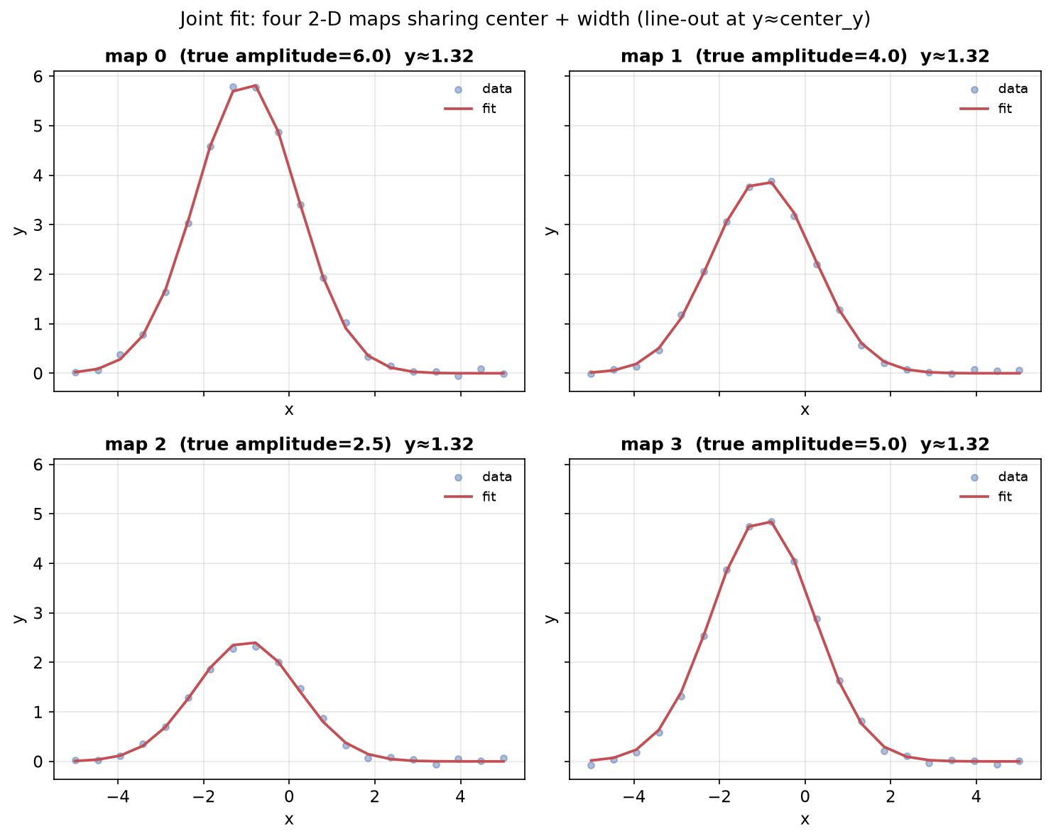
An illustrative 2-D multi-spectrum case (synthetic, one geometry): N 2-D gaussian2d spectra that differ only in amplitude are fitted jointly. The shared peak center and widths are constrained by all four maps at once; each map contributes its own amplitude. This demonstrates the mechanism (SP-3) in one representative seeded instance — not a sweep across geometries or noise levels.

def synthesize_shared_shape_maps() -> tuple[
    list[MeasurementData],
    np.ndarray,
    np.ndarray,
    np.ndarray,
    tuple[float, float, float, float],
    list[float],
]:
    """Synthesize four 2-D Gaussian maps sharing center and both widths.

    Builds one shared 20x20 (x, y) grid, then four maps with an identical
    peak center/width but a different amplitude each, plus independent
    Gaussian measurement noise. Returns ``(datasets, gx, gy, xx, (cx, cy, sx,
    sy), amps_true)`` — everything the graph-building, reporting, and
    plotting steps below need.
    """
    nx = ny = 20
    gx = np.linspace(-5.0, 5.0, nx)
    gy = np.linspace(-5.0, 5.0, ny)
    xx, yy = np.meshgrid(gx, gy)
    coords = np.column_stack([xx.ravel(), yy.ravel()])

    # Ground-truth shared shape; only amplitude varies across the four maps.
    cx, cy, sx, sy = -1.0, 1.5, 1.2, 0.9
    amps_true = [6.0, 4.0, 2.5, 5.0]
    rng = np.random.default_rng(3)

    def g2d(a: float) -> np.ndarray:
        return a * np.exp(-0.5 * (((xx - cx) / sx) ** 2 + ((yy - cy) / sy) ** 2))

    datasets = [
        MeasurementData(
            x=coords.tolist(),
            y=(g2d(a) + rng.normal(0.0, 0.05, xx.shape)).ravel().tolist(),
        )
        for a in amps_true
    ]
    return datasets, gx, gy, xx, (cx, cy, sx, sy), amps_true


datasets, gx, gy, xx, (cx, cy, sx, sy), amps_true = synthesize_shared_shape_maps()

Same pattern as the 1-D case, scaled up: four replicas of one gaussian2d node, this time with shared_local_params tying all four shape parameters (center_x, center_y, sigma_x, sigma_y) at once, leaving only amplitude free per map.

def build_graph(n_slices: int) -> GlobalFitGraph:
    """Build a GlobalFitGraph: one local 2-D Gaussian peak replicated per map.

    ``global_nodes=[]`` and ``local_nodes=[<one peak>]`` means the peak is
    replicated once per map (``n_slices``). ``shared_local_params`` ties
    ``center_x``, ``center_y``, ``sigma_x``, ``sigma_y`` across all replicas
    via a hard ``ExprEdge`` constraint each; ``amplitude`` stays free per map.
    """

    def peak() -> ModelNodeSpec:
        return ModelNodeSpec(
            id="pk",
            model_type=ModelType.GAUSSIAN2D,
            parameters={
                "amplitude": Parameter(value=3.0, min=0.0),
                "center_x": Parameter(value=-0.5),
                "center_y": Parameter(value=1.0),
                "sigma_x": Parameter(value=1.0, min=0.1),
                "sigma_y": Parameter(value=1.0, min=0.1),
            },
        )

    return GlobalFitGraph(
        global_nodes=[],
        local_nodes=[peak()],
        n_slices=n_slices,
        shared_local_params=["center_x", "center_y", "sigma_x", "sigma_y"],
    )


graph = build_graph(len(datasets))

The joint solve now spans 1600 data points across all four maps but only 8 free parameters — the shared shape sees four times the evidence a single map's fit would.

def fit_datasets(graph: GlobalFitGraph, datasets: list[MeasurementData]) -> FitResult:
    """Run the joint solve: one residual vector of all four maps at once."""
    return graph.fit(datasets)


result = fit_datasets(graph, datasets)
p = {k: v.value for k, v in result.parameters.items()}

Same tie guarantee as before, just across four shared parameters instead of one: each drift below is 0.0 because the constraint is hard, not approximate.

def report_result(
    result: FitResult,
    p: dict[str, float],
    cx: float,
    cy: float,
    sx: float,
    sy: float,
    amps_true: list[float],
) -> None:
    """Print success/R², recovered shared shape, per-map amplitudes, and tie drift.

    The tie drift for each shared parameter (the max absolute difference from
    slice 0's value, across the remaining slices) is expected to be 0.0 to
    machine precision — the engine enforces every ``shared_local_params`` tie
    as a hard ``ExprEdge`` constraint, not a soft penalty.
    """
    print(f"Success: {result.success}")
    print(f"R²:      {result.r_squared:.6f}")
    print()
    print("Recovered shared params (all four maps contribute):")
    print(f"  center_x = {p['pk_s0.center_x']:.4f}  (true {cx})")
    print(f"  center_y = {p['pk_s0.center_y']:.4f}  (true {cy})")
    print(f"  sigma_x  = {p['pk_s0.sigma_x']:.4f}  (true {sx})")
    print(f"  sigma_y  = {p['pk_s0.sigma_y']:.4f}  (true {sy})")
    print()
    print("Per-map amplitudes:")
    for i, a_true in enumerate(amps_true):
        print(
            f"  slice {i}: amplitude = {p[f'pk_s{i}.amplitude']:.4f}  (true {a_true})",
        )
    print()
    print("Tie drift across slices (must be 0.0):")
    for param in ["center_x", "center_y", "sigma_x", "sigma_y"]:
        drift = max(
            abs(p[f"pk_s{i}.{param}"] - p["pk_s0." + param]) for i in range(1, len(amps_true))
        )
        print(f"  {param}: {drift:.2e}")


report_result(result, p, cx, cy, sx, sy, amps_true)

What just happened¶

Four 2-D spectra — each is a 20×20 gaussian2d map with the same peak center and widths but a different amplitude. The true parameters are center_x = −1.0, center_y = 1.5, sigma_x = 1.2, sigma_y = 0.9.
Shared shape, free amplitude — shared_local_params ties center_x, center_y, sigma_x, sigma_y across all four dataset replicas. Each replica's amplitude remains free.
One joint solve — the optimizer minimizes a residual vector of length 4 × 400 = 1600 data points simultaneously, with 4 (shared shape) + 4 (per-slice amplitudes) = 8 free parameters.
Tie drift is 0.0 in this run — within this solve the shared parameters are identical across slices (not approximately equal), because the engine enforces each tie as a hard constraint (ExprEdge), not a soft penalty. The printed drift of 0.0 is a property of how the constraint is implemented, reported for the specific geometry shown above.

Why this works¶

One simultaneous joint solve is strictly better than N independent fits: shared parameters are constrained by all data points at once, giving a more precise estimate and ensuring consistency.

Typical use cases: temperature-dependent measurements sharing a peak position; a series of samples sharing a calibrated instrument response; spatial maps sharing center and width but varying amplitude per location.

Contrast with shared_params.md (which ties parameters across peaks within one spectrum; this file ties parameters across datasets).

Benchmark UI status

The corresponding global_fit contract field is now rendered in the production web UI as a "global-fit-showcase" panel within the Evidence destination's "Native showcases" section. The capability lives in the fitting engine (GlobalFitGraph) and is exercised by tests, and the benchmark showcase is displayed alongside other native multi-dataset fitting demonstrations.

Honest naming note¶

This capability was previously misnamed time_resolved in the benchmark contract. That name implied a time axis, but the mechanism is a general shared-model multi-spectrum joint fit: time is just one incidental axis interpretation. The contract field was renamed global_fit (classes GlobalFit / GlobalFitSlice, axis fields dataset_axis / coord / axis_label) in schema version 1.6.

Multi-Dataset Joint Fitting¶

1-D example: local peaks with a shared line width¶

What just happened¶

2-D multi-spectrum example: four different maps sharing center and width¶

What just happened¶

Why this works¶

Honest naming note¶

See also¶