Parameter Confidence Intervals
Synthetic example
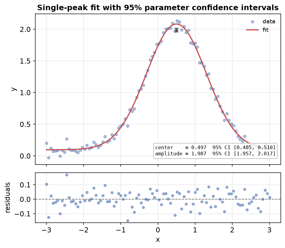
The fixture below is a single seeded Gaussian peak with known truth parameters — chosen so the reported 95% confidence interval can be checked against a known answer, not a sweep proving Wald-interval coverage holds generally across noise levels or parameter regimes.
Context
When to use this pattern. A point estimate and its stderr are useful,
but reporting a 95% confidence interval is usually what a downstream
consumer (a paper, a report, a decision) actually needs. This example turns
every fitted parameter's stderr into a 95% confidence interval using the
standard normal ("Wald") approximation, and annotates it directly on the
plot for the two parameters most people care about — a peak's center and
amplitude.
Quick example
def synthesize_data() -> tuple[np.ndarray, np.ndarray]:
    """Synthesize a single Gaussian peak on a constant background (with noise).

    Same shape as fitting.py, extended here with confidence-interval
    reporting downstream.
    """
    rng = np.random.default_rng(3)
    x = np.linspace(-3, 3, 100)
    peak = 2.0 * np.exp(-0.5 * ((x - 0.5) / 0.8) ** 2)
    background = 0.1
    noise = rng.normal(0, 0.05, len(x))
    y = peak + background + noise
    return x, y


x, y = synthesize_data()
Nothing new here versus fitting.md — same peak-plus-background shape.
def build_graph() -> FitGraph:
    """Build a FitGraph: one Gaussian peak + one constant background."""
    return FitGraph(
        nodes=[
            ModelNodeSpec(
                id="peak",
                model_type=ModelType.GAUSSIAN,
                parameters={
                    "amplitude": Parameter(value=1.5),
                    "center": Parameter(value=0.0),
                    "sigma": Parameter(value=0.5, min=1e-3),
                },
            ),
            ModelNodeSpec(
                id="bg",
                model_type=ModelType.CONSTANT,
                parameters={"c": Parameter(value=0.0)},
            ),
        ],
    )


graph = build_graph()
Same solver, same call shape as fitting.md too — the interesting part
starts once result.parameters is in hand.
def run_fit(graph: FitGraph, x: np.ndarray, y: np.ndarray) -> FitResult:
    """Wrap the measurement data and invoke the Levenberg-Marquardt solver."""
    data = MeasurementData(x=x.tolist(), y=y.tolist())
    return fit(graph, data)


result = run_fit(graph, x, y)
stderr alone is a \(1\sigma\) standard error, not an interval — it needs scaling
by the standard normal's two-sided 95% critical value (\(Z_{95} \approx 1.96\)) to
become a Wald confidence interval, and that scaling is a linear
approximation around the fitted optimum, not an exact bound.
def build_confidence_intervals(result: FitResult) -> dict[str, tuple[float, float]]:
    """Print success/R², then turn each parameter's ``stderr`` into a 95% Wald CI.

    ``ci_95 = value +/- Z_95 * stderr`` (see the module docstring for the
    linear-approximation caveat). Asserts the fit succeeded and every
    returned CI is properly ordered (lo <= hi).
    """
    print(f"Success: {result.success}")
    print(f"R²: {result.r_squared:.6f}")
    print()

    print(
        f"{'parameter':18s} {'value':>10s} {'stderr':>10s} {'95% CI low':>12s} {'95% CI high':>12s}",
    )
    ci_by_param: dict[str, tuple[float, float]] = {}
    for name, param in sorted(result.parameters.items()):
        if param.stderr is None:
            print(
                f"{name:18s} {param.value:10.4f} {'n/a':>10s} {'n/a':>12s} {'n/a':>12s}",
            )
            continue
        half_width = Z_95 * param.stderr
        ci_lo, ci_hi = param.value - half_width, param.value + half_width
        ci_by_param[name] = (ci_lo, ci_hi)
        print(
            f"{name:18s} {param.value:10.4f} {param.stderr:10.4f} {ci_lo:12.4f} {ci_hi:12.4f}",
        )

    assert result.success
    assert all(lo <= hi for lo, hi in ci_by_param.values()), "CI bounds must be ordered"
    return ci_by_param


ci_by_param = build_confidence_intervals(result)
What just happened
-
Fit as usual — a single Gaussian peak plus a constant background, the same shape as Single-Dataset Fitting.
-
From
stderrto a 95% CI — for each free parameter, \(ci_{95} = \text{value} \pm 1.959964 \cdot \text{stderr}\) (1.959964is the two-sided 95% critical value of the standard normal distribution). This is a linear approximation around the fitted optimum: it assumes the parameter's sampling distribution is well described by a normal distribution with the reported variance. That holds well for well-determined, close-to-linear problems like this one, but can understate or misshape the true interval for a strongly nonlinear or poorly-determined parameter. -
stderrcan beNone. It is derived from the Jacobian at the fitted optimum, and that derivation is refused rather than returning a bogus number when the Jacobian is empty, rank-deficient, or otherwise ill-conditioned (overlapping/redundant peaks, or a parameter that barely moves the model, are the usual causes) —ParameterResult.stderrisNonein that case, not a step this tutorial's pattern can silently skip over. Check forNonebefore computing a CI from it on real, more-degenerate data than this example's clean single peak. -
Not covered here: profile-likelihood intervals. A tighter alternative traces the actual \(\chi^2\) surface as one parameter is stepped away from its optimum, rather than assuming a local quadratic (normal) shape around it. That capability is not yet demonstrated by a gallery tutorial — this example is scoped to the
stderr-based Wald interval, which is whatFitResultexposes directly. -
Visual reporting — the fitted curve is plotted as usual, with the peak apex's
centerandamplitude95% CIs drawn as error-bar whiskers and printed on the plot, alongside a full table (all four free parameters) printed to stdout.
See also
- Related examples:
fitting.md(the base single-peak pattern),varpro_vs_lm.md(solver comparison on a separable fit). - Reference: Solver — Post-fit statistics
for how
stderrandcovarianceare derived. - API docs:
FitResult,ParameterResult.