Many Local Minima Functions
Ackley Function
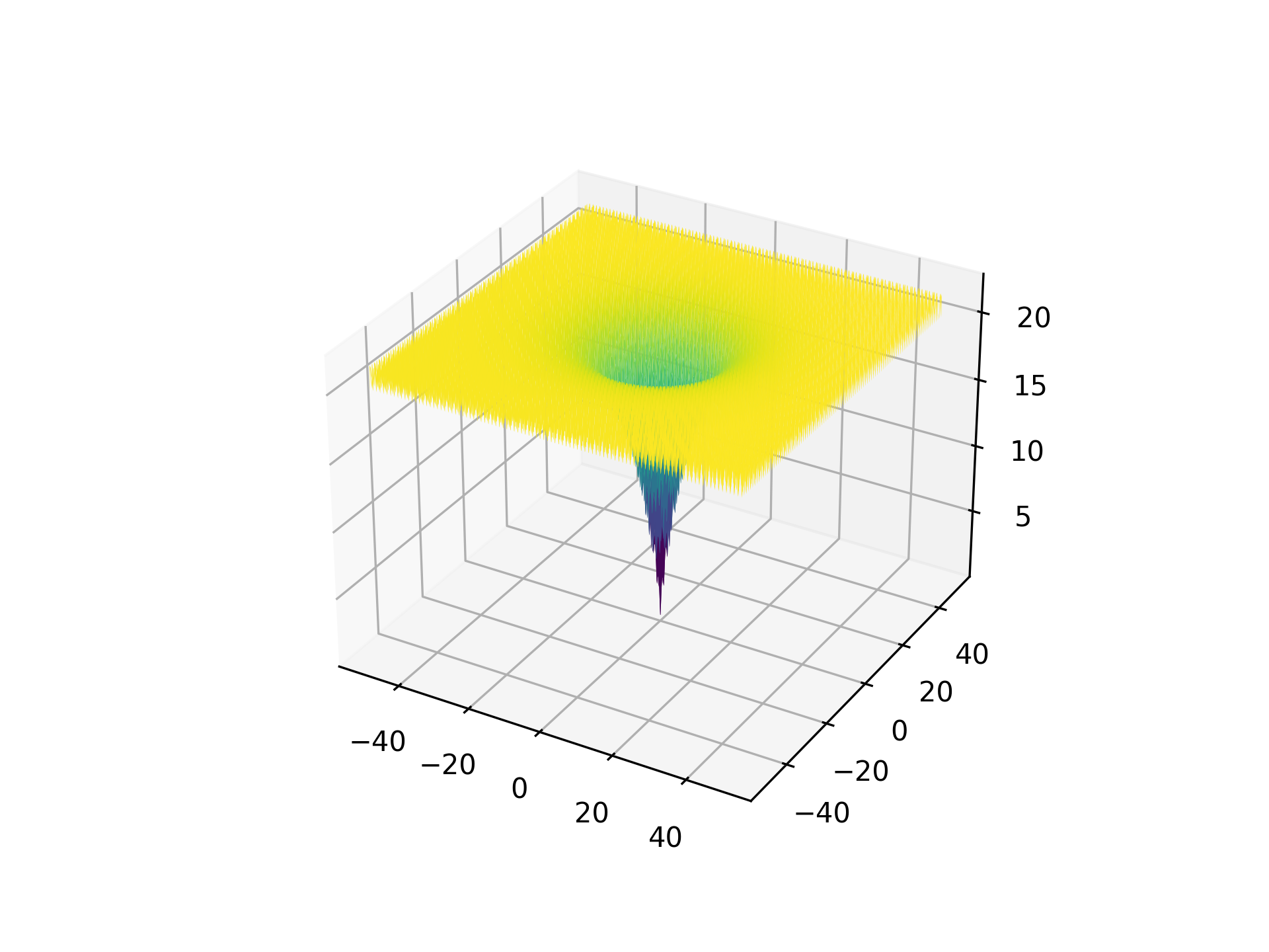
Ackley function.
The Ackley function is a multi-dimensional function with many local minima.
Examples:
>>> import matplotlib.pyplot as plt
>>> import numpy as np
>>> from umf.functions.optimization.many_local_minima import AckleyFunction
>>> x = np.linspace(-50, 50, 1000)
>>> y = np.linspace(-50, 50, 1000)
>>> X, Y = np.meshgrid(x, y)
>>> Z = AckleyFunction(X, Y).__eval__
>>> fig = plt.figure()
>>> ax = fig.add_subplot(111, projection="3d")
>>> _ = ax.plot_surface(X, Y, Z, cmap="viridis")
>>> plt.savefig("AckleyFunction.png", dpi=300, transparent=True)
Notes
The Ackley function is defined as:
Reference: Original implementation can be found here.
Parameters:
| Name | Type | Description | Default |
|---|---|---|---|
*x | UniversalArray | Input data, which can be one, two, three, or higher dimensional. | () |
alpha | float | Scaling factor. Default is 20.0. | 20.0 |
beta | float | Scaling factor. Default is 0.2. | 0.2 |
gamma | float | Scaling factor. Default is 2.0 * np.pi. | 2.0 * pi |
Source code in src/umf/functions/optimization/many_local_minima.py
class AckleyFunction(OptFunction):
    r"""Ackley function.

    The Ackley function is a multi-dimensional function with many local minima.

    Examples:
        >>> import matplotlib.pyplot as plt
        >>> import numpy as np
        >>> from umf.functions.optimization.many_local_minima import AckleyFunction
        >>> x = np.linspace(-50, 50, 1000)
        >>> y = np.linspace(-50, 50, 1000)
        >>> X, Y = np.meshgrid(x, y)
        >>> Z = AckleyFunction(X, Y).__eval__
        >>> fig = plt.figure()
        >>> ax = fig.add_subplot(111, projection="3d")
        >>> _ = ax.plot_surface(X, Y, Z, cmap="viridis")
        >>> plt.savefig("AckleyFunction.png", dpi=300, transparent=True)

    Notes:
        The Ackley function is defined as:

        $$
            f(x) = -\alpha \exp \left( -\beta \sqrt{\frac{1}{n} \sum_{i=1}^n x_i^2}
              \right) - \exp \left( \frac{1}{n} \sum_{i=1}^n \cos(\gamma x_i)
              \right) + e + \alpha
        $$

        > Reference: Original implementation can be found
        > [here](https://www.sfu.ca/~ssurjano/ackley.html).

    Args:
        *x (UniversalArray): Input data, which can be one, two, three, or higher
             dimensional.
        alpha (float): Scaling factor. Default is 20.0.
        beta (float): Scaling factor. Default is 0.2.
        gamma (float): Scaling factor. Default is 2.0 * np.pi.
    """

    def __init__(
        self,
        *x: UniversalArray,
        alpha: float = 20.0,
        beta: float = 0.2,
        gamma: float = 2.0 * np.pi,
    ) -> None:
        """Initialize the function."""
        super().__init__(*x)
        self._alpha = alpha
        self._beta = beta
        self._gamma = gamma

    @property
    def __eval__(self) -> UniversalArray:
        """Evaluate Ackley function at x.

        Returns:
            UniversalArray: Function values as numpy arrays.
        """
        sum_1 = np.zeros_like(self._x[0])
        sum_2 = np.zeros_like(self._x[0])

        for _i, _x in enumerate(self._x, start=1):
            # Calculate sum of squares of x values
            sum_1 += _x**2
            # Calculate sum of cosines of x values
            sum_2 += np.cos(self._gamma * _x)

        # Calculate exponential terms
        terms_1 = -self._alpha * np.exp(-self._beta * np.sqrt(1 / _i * sum_1))
        terms_2 = -np.exp(1 / _i * sum_2)

        # Calculate Ackley function value
        terms_3 = np.e + self._alpha
        return terms_1 + terms_2 + terms_3

    @property
    def __minima__(self) -> MinimaAPI:
        """Return the minima of the Ackley function."""
        return MinimaAPI(f_x=0.0, x=tuple(np.zeros_like(self._x[0])))
__eval__ property ¶Evaluate Ackley function at x.
Returns:
| Name | Type | Description |
|---|---|---|
UniversalArray | UniversalArray | Function values as numpy arrays. |
__minima__ property ¶Return the minima of the Ackley function.
__init__(*x, alpha=20.0, beta=0.2, gamma=2.0 * np.pi) ¶Initialize the function.
Source code in src/umf/functions/optimization/many_local_minima.py
 |
Bukin Function N. 6
Bukin function number 6.
The Bukin function number 6 is a two-dimensional function with many local minima.
Examples:
>>> import matplotlib.pyplot as plt
>>> import numpy as np
>>> from umf.functions.optimization.many_local_minima import BukinN6Function
>>> x = np.linspace(-15, 5, 1000)
>>> y = np.linspace(-3, 3, 1000)
>>> X, Y = np.meshgrid(x, y)
>>> Z = BukinN6Function(X, Y).__eval__
>>> fig = plt.figure()
>>> ax = fig.add_subplot(111, projection="3d")
>>> _ = ax.plot_surface(X, Y, Z, cmap="viridis")
>>> plt.savefig("BukinN6Function.png", dpi=300, transparent=True)
Notes
The Bukin function number 6 is defined as:
Reference: Original implementation can be found here.
Parameters:
| Name | Type | Description | Default |
|---|---|---|---|
*x | UniversalArray | Input data, which has to be two dimensional. | () |
Source code in src/umf/functions/optimization/many_local_minima.py
class BukinN6Function(OptFunction):
    r"""Bukin function number 6.

    The Bukin function number 6 is a two-dimensional function with many local minima.

    Examples:
        >>> import matplotlib.pyplot as plt
        >>> import numpy as np
        >>> from umf.functions.optimization.many_local_minima import BukinN6Function
        >>> x = np.linspace(-15, 5, 1000)
        >>> y = np.linspace(-3, 3, 1000)
        >>> X, Y = np.meshgrid(x, y)
        >>> Z = BukinN6Function(X, Y).__eval__
        >>> fig = plt.figure()
        >>> ax = fig.add_subplot(111, projection="3d")
        >>> _ = ax.plot_surface(X, Y, Z, cmap="viridis")
        >>> plt.savefig("BukinN6Function.png", dpi=300, transparent=True)

    Notes:
        The Bukin function number 6 is defined as:

        $$
            f(x) = 100 \sqrt{\left| y - 0.01 x^2 \right|} +
            0.01 \left| x + 10 \right|
        $$

        > Reference: Original implementation can be found
        > [here](https://www.sfu.ca/~ssurjano/bukin6.html).

    Args:
        *x (UniversalArray): Input data, which has to be two dimensional.
    """

    def __init__(self, *x: UniversalArray) -> None:
        """Initialize the function."""
        if len(x) != __2d__:
            raise OutOfDimensionError(
                function_name="Bukin",
                dimension=__2d__,
            )
        super().__init__(*x)

    @property
    def __eval__(self) -> UniversalArray:
        """Evaluate Bukin function at x.

        Returns:
            UniversalArray: Function values as numpy arrays.
        """
        x_1 = self._x[0]
        x_2 = self._x[1]

        term_1 = 100 * np.sqrt(np.abs(x_2 - 0.01 * x_1**2))
        term_2 = 0.01 * np.abs(x_1 + 10)

        return term_1 + term_2

    @property
    def __minima__(self) -> MinimaAPI:
        """Return the minima of the function.

        Returns:
            MinimaAPI: MinimaAPI object containing the minima of the function.
        """
        return MinimaAPI(
            f_x=0.0,
            x=(-10.0, 1.0),
        )
__eval__ property ¶Evaluate Bukin function at x.
Returns:
| Name | Type | Description |
|---|---|---|
UniversalArray | UniversalArray | Function values as numpy arrays. |
__minima__ property ¶Return the minima of the function.
Returns:
| Name | Type | Description |
|---|---|---|
MinimaAPI | MinimaAPI | MinimaAPI object containing the minima of the function. |
__init__(*x) ¶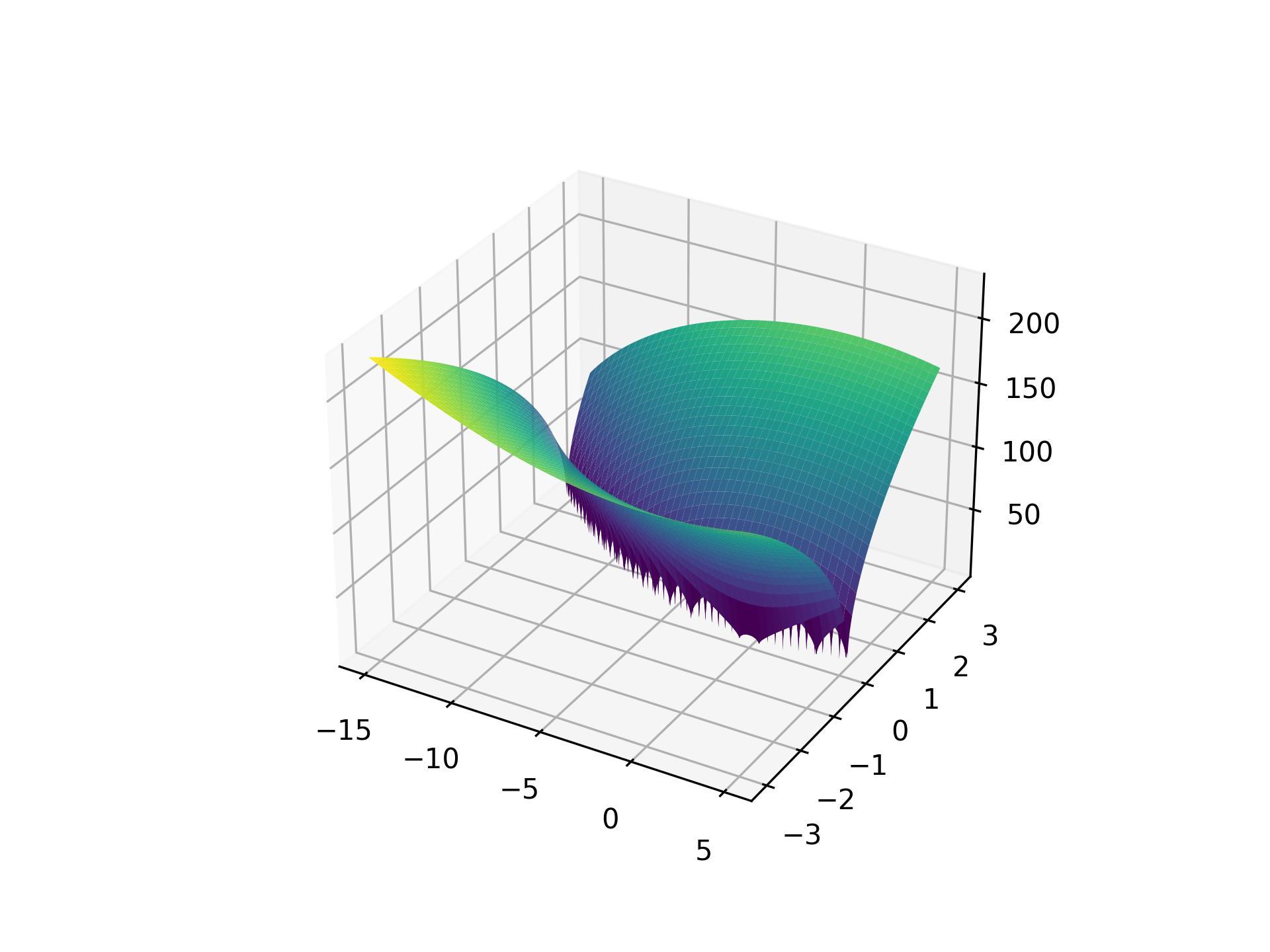 |
Cross-in-Tray Function
Cross-in-tray function.
The Cross-in-tray function is a two-dimensional function with many local minima.
Examples:
>>> import matplotlib.pyplot as plt
>>> import numpy as np
>>> from umf.functions.optimization.many_local_minima import CrossInTrayFunction
>>> x = np.linspace(-10, 10, 1000)
>>> y = np.linspace(-10, 10, 1000)
>>> X, Y = np.meshgrid(x, y)
>>> Z = CrossInTrayFunction(X, Y).__eval__
>>> fig = plt.figure()
>>> ax = fig.add_subplot(111, projection="3d")
>>> _ = ax.plot_surface(X, Y, Z, cmap="viridis")
>>> plt.savefig("CrossInTrayFunction.png", dpi=300, transparent=True)
Notes
The Cross-in-tray function is defined as:
Reference: Original implementation can be found here.
Parameters:
| Name | Type | Description | Default |
|---|---|---|---|
*x | UniversalArray | Input data, which has to be two dimensional. | () |
Source code in src/umf/functions/optimization/many_local_minima.py
class CrossInTrayFunction(OptFunction):
    r"""Cross-in-tray function.

    The Cross-in-tray function is a two-dimensional function with many local minima.

    Examples:
        >>> import matplotlib.pyplot as plt
        >>> import numpy as np
        >>> from umf.functions.optimization.many_local_minima import CrossInTrayFunction
        >>> x = np.linspace(-10, 10, 1000)
        >>> y = np.linspace(-10, 10, 1000)
        >>> X, Y = np.meshgrid(x, y)
        >>> Z = CrossInTrayFunction(X, Y).__eval__
        >>> fig = plt.figure()
        >>> ax = fig.add_subplot(111, projection="3d")
        >>> _ = ax.plot_surface(X, Y, Z, cmap="viridis")
        >>> plt.savefig("CrossInTrayFunction.png", dpi=300, transparent=True)

    Notes:
        The Cross-in-tray function is defined as:

        $$
            f(x) = -0.0001 \cdot \left( \left| \sin(x_1) \sin(x_2)
            \exp \left( \left| 100 - \sqrt{x_1^2 + x_2^2} / \pi \right| \right) \right|
            + 1 \right)^{0.1}
        $$

        > Reference: Original implementation can be found
        > [here](https://www.sfu.ca/~ssurjano/crossit.html).


    Args:
        *x (UniversalArray): Input data, which has to be two dimensional.
    """

    def __init__(self, *x: UniversalArray) -> None:
        """Initialize the function."""
        if len(x) != __2d__:
            raise OutOfDimensionError(
                function_name="Cross-in-tray",
                dimension=__2d__,
            )
        super().__init__(*x)

    @property
    def __eval__(self) -> UniversalArray:
        """Evaluate Cross-in-tray function at x.

        Returns:
            UniversalArray: Function values as numpy arrays.
        """
        x_1 = self._x[0]
        x_2 = self._x[1]

        term_1 = np.sin(x_1) * np.sin(x_2)
        term_2 = np.exp(np.abs(100 - np.sqrt(x_1**2 + x_2**2) / np.pi))
        return -0.0001 * np.abs(term_1 * term_2 + 1) ** 0.1

    @property
    def __minima__(self) -> MinimaAPI:
        """Return the minima of the function.

        Returns:
            MinimaAPI: MinimaAPI object containing the minima of the function.
        """
        return MinimaAPI(
            f_x=-2.06261,
            x=tuple(
                np.array([1.34941, 1.34941]),
                np.array([-1.34941, -1.34941]),
                np.array([1.34941, -1.34941]),
                np.array([-1.34941, 1.34941]),
            ),
        )
__eval__ property ¶Evaluate Cross-in-tray function at x.
Returns:
| Name | Type | Description |
|---|---|---|
UniversalArray | UniversalArray | Function values as numpy arrays. |
__minima__ property ¶Return the minima of the function.
Returns:
| Name | Type | Description |
|---|---|---|
MinimaAPI | MinimaAPI | MinimaAPI object containing the minima of the function. |
__init__(*x) ¶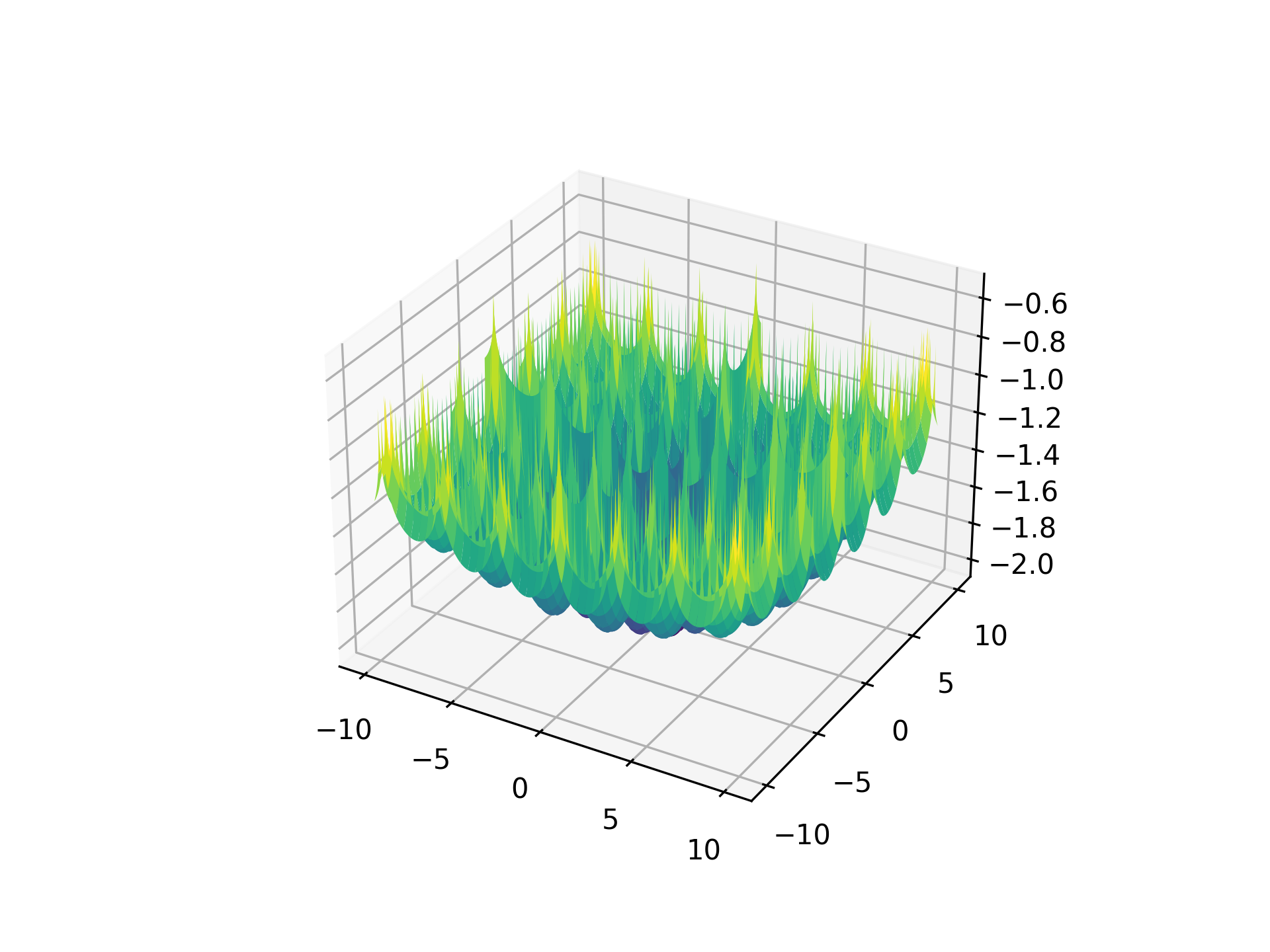 |
Drop Wave Function
Drop-wave function.
The Drop-wave function is a two-dimensional function with many local minima.
Examples:
>>> import matplotlib.pyplot as plt
>>> import numpy as np
>>> from umf.functions.optimization.many_local_minima import DropWaveFunction
>>> x = np.linspace(-5, 5, 1000)
>>> y = np.linspace(-5, 5, 1000)
>>> X, Y = np.meshgrid(x, y)
>>> Z = DropWaveFunction(X, Y).__eval__
>>> fig = plt.figure()
>>> ax = fig.add_subplot(111, projection="3d")
>>> _ = ax.plot_surface(X, Y, Z, cmap="viridis")
>>> plt.savefig("DropWaveFunction.png", dpi=300, transparent=True)
Notes
The Drop-wave function is defined as:
Reference: Original implementation can be found here.
Parameters:
| Name | Type | Description | Default |
|---|---|---|---|
*x | UniversalArray | Input data, which has to be two dimensional. | () |
Source code in src/umf/functions/optimization/many_local_minima.py
class DropWaveFunction(OptFunction):
    r"""Drop-wave function.

    The Drop-wave function is a two-dimensional function with many local minima.

    Examples:
        >>> import matplotlib.pyplot as plt
        >>> import numpy as np
        >>> from umf.functions.optimization.many_local_minima import DropWaveFunction
        >>> x = np.linspace(-5, 5, 1000)
        >>> y = np.linspace(-5, 5, 1000)
        >>> X, Y = np.meshgrid(x, y)
        >>> Z = DropWaveFunction(X, Y).__eval__
        >>> fig = plt.figure()
        >>> ax = fig.add_subplot(111, projection="3d")
        >>> _ = ax.plot_surface(X, Y, Z, cmap="viridis")
        >>> plt.savefig("DropWaveFunction.png", dpi=300, transparent=True)

    Notes:
        The Drop-wave function is defined as:

        $$
            f(x) = -\left( 1 + \cos(12 \sqrt{x_1^2 + x_2^2}) \right)
            / (0.5(x_1^2 + x_2^2) + 2)
        $$

        > Reference: Original implementation can be found
        > [here](https://www.sfu.ca/~ssurjano/drop.html).

    Args:
        *x (UniversalArray): Input data, which has to be two dimensional.
    """

    def __init__(self, *x: UniversalArray) -> None:
        """Initialize the function."""
        if len(x) != __2d__:
            raise OutOfDimensionError(
                function_name="Drop-wave",
                dimension=__2d__,
            )
        super().__init__(*x)

    @property
    def __eval__(self) -> UniversalArray:
        """Evaluate Drop-wave function at x.

        Returns:
            UniversalArray: Function values as numpy arrays.
        """
        x_1 = self._x[0]
        x_2 = self._x[1]

        term_1 = 12 * np.sqrt(x_1**2 + x_2**2)
        term_2 = 0.5 * (x_1**2 + x_2**2) + 2

        return -((1 + np.cos(term_1)) / term_2)

    @property
    def __minima__(self) -> MinimaAPI:
        """Return the minima of the function.

        Returns:
            MinimaAPI: MinimaAPI object containing the minima of the function.
        """
        return MinimaAPI(f_x=-1.0, x=tuple(0.0, 0.0))
__eval__ property ¶Evaluate Drop-wave function at x.
Returns:
| Name | Type | Description |
|---|---|---|
UniversalArray | UniversalArray | Function values as numpy arrays. |
__minima__ property ¶Return the minima of the function.
Returns:
| Name | Type | Description |
|---|---|---|
MinimaAPI | MinimaAPI | MinimaAPI object containing the minima of the function. |
__init__(*x) ¶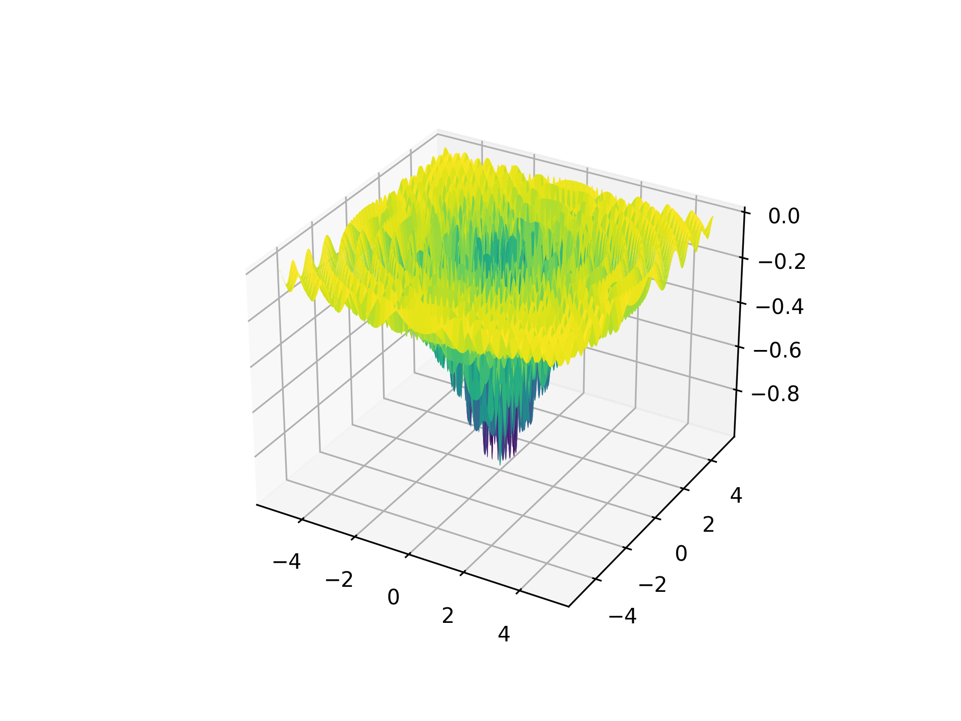 |
Egg Holder Function
Egg-holder function.
The Egg-holder function is a two-dimensional function with many local minima.
Examples:
>>> import matplotlib.pyplot as plt
>>> import numpy as np
>>> from umf.functions.optimization.many_local_minima import EggHolderFunction
>>> x = np.linspace(-512, 512, 1000)
>>> y = np.linspace(-512, 512, 1000)
>>> X, Y = np.meshgrid(x, y)
>>> Z = EggHolderFunction(X, Y).__eval__
>>> fig = plt.figure()
>>> ax = fig.add_subplot(111, projection="3d")
>>> _ = ax.plot_surface(X, Y, Z, cmap="viridis")
>>> plt.savefig("EggHolderFunction.png", dpi=300, transparent=True)
Notes
The Egg-holder function is defined as:
Reference: Original implementation can be found here.
Parameters:
| Name | Type | Description | Default |
|---|---|---|---|
*x | UniversalArray | Input data, which has to be two dimensional. | () |
Source code in src/umf/functions/optimization/many_local_minima.py
class EggHolderFunction(OptFunction):
    r"""Egg-holder function.

    The Egg-holder function is a two-dimensional function with many local minima.

    Examples:
        >>> import matplotlib.pyplot as plt
        >>> import numpy as np
        >>> from umf.functions.optimization.many_local_minima import EggHolderFunction
        >>> x = np.linspace(-512, 512, 1000)
        >>> y = np.linspace(-512, 512, 1000)
        >>> X, Y = np.meshgrid(x, y)
        >>> Z = EggHolderFunction(X, Y).__eval__
        >>> fig = plt.figure()
        >>> ax = fig.add_subplot(111, projection="3d")
        >>> _ = ax.plot_surface(X, Y, Z, cmap="viridis")
        >>> plt.savefig("EggHolderFunction.png", dpi=300, transparent=True)

    Notes:
        The Egg-holder function is defined as:

        $$
            f(x) = -(x_2 + 47) \sin \left( \sqrt{\left| x_2 + \frac{x_1}{2}
            + 47 \right|} \right) - x_1 \sin \left( \sqrt{\left| x_1
            - (x_2 + 47) \right|} \right)
        $$

        > Reference: Original implementation can be found
        > [here](https://www.sfu.ca/~ssurjano/egg.html).


    Args:
        *x (UniversalArray): Input data, which has to be two dimensional.
    """

    def __init__(self, *x: UniversalArray) -> None:
        """Initialize the function."""
        if len(x) != __2d__:
            raise OutOfDimensionError(
                function_name="Egg-holder",
                dimension=__2d__,
            )
        super().__init__(*x)

    @property
    def __eval__(self) -> UniversalArray:
        """Evaluate Egg-holder function at x.

        Returns:
            UniversalArray: Function values as numpy arrays.
        """
        x_1 = self._x[0]
        x_2 = self._x[1]

        term_1 = np.sqrt(np.abs(x_2 + 47 + x_1 / 2))
        term_2 = np.sqrt(np.abs(x_1 - (x_2 + 47)))

        return -(x_2 + 47) * np.sin(term_1) - x_1 * np.sin(term_2)

    @property
    def __minima__(self) -> MinimaAPI:
        """Return the minima of the function.

        Returns:
            MinimaAPI: MinimaAPI object containing the minima of the function.
        """
        return MinimaAPI(f_x=-959.6407, x=tuple(512, 404.2319))
__eval__ property ¶Evaluate Egg-holder function at x.
Returns:
| Name | Type | Description |
|---|---|---|
UniversalArray | UniversalArray | Function values as numpy arrays. |
__minima__ property ¶Return the minima of the function.
Returns:
| Name | Type | Description |
|---|---|---|
MinimaAPI | MinimaAPI | MinimaAPI object containing the minima of the function. |
__init__(*x) ¶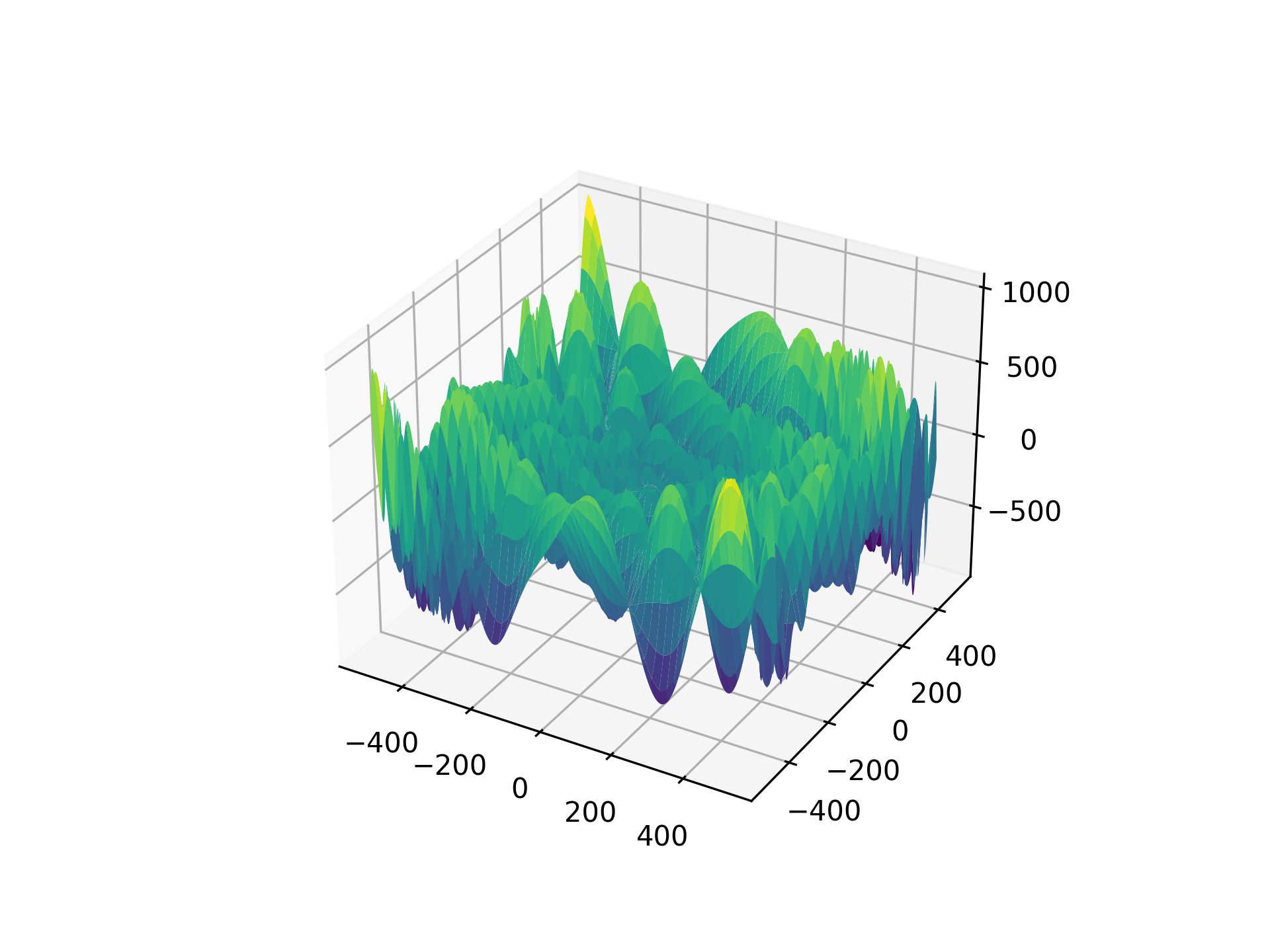 |
Griewank Function
Griewank function.
The Griewank function is a multi-dimensional function with many local minima.
Examples:
>>> import matplotlib.pyplot as plt
>>> import numpy as np
>>> from umf.functions.optimization.many_local_minima import GriewankFunction
>>> x = np.linspace(-50, 50, 1000)
>>> y = np.linspace(-50, 50, 1000)
>>> X, Y = np.meshgrid(x, y)
>>> Z = GriewankFunction(X, Y).__eval__
>>> fig = plt.figure()
>>> ax = fig.add_subplot(111, projection="3d")
>>> _ = ax.plot_surface(X, Y, Z, cmap="viridis")
>>> plt.savefig("GriewankFunction.png", dpi=300, transparent=True)
Notes
The Griewank function is defined as:
Reference: Original implementation can be found here.
Parameters:
| Name | Type | Description | Default |
|---|---|---|---|
*x | UniversalArray | Input data, which has to be two dimensional. | () |
Source code in src/umf/functions/optimization/many_local_minima.py
class GriewankFunction(OptFunction):
    r"""Griewank function.

    The Griewank function is a multi-dimensional function with many local minima.

    Examples:
        >>> import matplotlib.pyplot as plt
        >>> import numpy as np
        >>> from umf.functions.optimization.many_local_minima import GriewankFunction
        >>> x = np.linspace(-50, 50, 1000)
        >>> y = np.linspace(-50, 50, 1000)
        >>> X, Y = np.meshgrid(x, y)
        >>> Z = GriewankFunction(X, Y).__eval__
        >>> fig = plt.figure()
        >>> ax = fig.add_subplot(111, projection="3d")
        >>> _ = ax.plot_surface(X, Y, Z, cmap="viridis")
        >>> plt.savefig("GriewankFunction.png", dpi=300, transparent=True)

    Notes:
        The Griewank function is defined as:

        $$
            f(x) = \frac{1}{4000} \sum_{i=1}^n x_i^2 - \prod_{i=1}^n \cos
            \left( \frac{x_i}{\sqrt{i}} \right) + 1
        $$

        > Reference: Original implementation can be found
        > [here](https://www.sfu.ca/~ssurjano/griewank.html).

    Args:
        *x (UniversalArray): Input data, which has to be two dimensional.
    """

    @property
    def __eval__(self) -> UniversalArray:
        """Evaluate Griewank function at x.

        Returns:
            UniversalArray: Function values as numpy arrays.
        """
        sum_ = np.zeros_like(self._x[0])
        for i, x_i in enumerate(self._x, start=1):
            sum_ += 1 / 4000 * x_i**2
            if i == 1:
                prod_ = np.cos(x_i / np.sqrt(i))
            prod_ *= np.cos(x_i / np.sqrt(i))

        return sum_ - prod_ + 1

    @property
    def __minima__(self) -> MinimaAPI:
        """Return the minima of the function.

        Returns:
            MinimaAPI: MinimaAPI object containing the minima of the function.
        """
        return MinimaAPI(f_x=0, x=tuple(np.zeros_like(self._x[0])))
__eval__ property ¶Evaluate Griewank function at x.
Returns:
| Name | Type | Description |
|---|---|---|
UniversalArray | UniversalArray | Function values as numpy arrays. |
 |
Holder Table Function
Holder table function.
The Holder table function is a two-dimensional function with many local minima.
Examples:
>>> import matplotlib.pyplot as plt
>>> import numpy as np
>>> from umf.functions.optimization.many_local_minima import HolderTableFunction
>>> x = np.linspace(-10, 10, 1000)
>>> y = np.linspace(-10, 10, 1000)
>>> X, Y = np.meshgrid(x, y)
>>> Z = HolderTableFunction(X, Y).__eval__
>>> fig = plt.figure()
>>> ax = fig.add_subplot(111, projection="3d")
>>> _ = ax.plot_surface(X, Y, Z, cmap="viridis")
>>> plt.savefig("HolderTableFunction.png", dpi=300, transparent=True)
Notes
The Holder table function is defined as:
Reference: Original implementation can be found here.
Parameters:
| Name | Type | Description | Default |
|---|---|---|---|
*x | UniversalArray | Input data, which has to be two dimensional. | () |
Source code in src/umf/functions/optimization/many_local_minima.py
class HolderTableFunction(OptFunction):
    r"""Holder table function.

    The Holder table function is a two-dimensional function with many local minima.

    Examples:
        >>> import matplotlib.pyplot as plt
        >>> import numpy as np
        >>> from umf.functions.optimization.many_local_minima import HolderTableFunction
        >>> x = np.linspace(-10, 10, 1000)
        >>> y = np.linspace(-10, 10, 1000)
        >>> X, Y = np.meshgrid(x, y)
        >>> Z = HolderTableFunction(X, Y).__eval__
        >>> fig = plt.figure()
        >>> ax = fig.add_subplot(111, projection="3d")
        >>> _ = ax.plot_surface(X, Y, Z, cmap="viridis")
        >>> plt.savefig("HolderTableFunction.png", dpi=300, transparent=True)

    Notes:
        The Holder table function is defined as:

        $$
            f(x) = -\left| \sin(x_1) \cos(x_2) \exp \left| 1 - \sqrt{x_1^2 + x_2^2} /
            \pi \right| \right|
        $$

        > Reference: Original implementation can be found
        > [here](https://www.sfu.ca/~ssurjano/holder.html).

    Args:
        *x (UniversalArray): Input data, which has to be two dimensional.
    """

    def __init__(self, *x: UniversalArray) -> None:
        """Initialize the function."""
        if len(x) != __2d__:
            raise OutOfDimensionError(
                function_name="Holder table",
                dimension=__2d__,
            )
        super().__init__(*x)

    @property
    def __eval__(self) -> UniversalArray:
        """Evaluate Holder table function at x.

        Returns:
            UniversalArray: Function values as numpy arrays.
        """
        x_1 = self._x[0]
        x_2 = self._x[1]

        term_1 = np.sin(x_1) * np.cos(x_2)
        term_2 = np.abs(1 - np.sqrt(x_1**2 + x_2**2) / np.pi)
        term_3 = np.exp(term_2)

        return -np.abs(term_1 * term_3)

    @property
    def __minima__(self) -> MinimaAPI:
        """Return the minima of the function.

        Returns:
            MinimaAPI: MinimaAPI object containing the minima of the function.
        """
        return MinimaAPI(
            f_x=-19.2085,
            x=tuple(
                np.array([8.05502, 9.66459]),
                np.array([8.05502, -9.66459]),
                np.array([-8.05502, 9.66459]),
                np.array([-8.05502, -9.66459]),
            ),
        )
__eval__ property ¶Evaluate Holder table function at x.
Returns:
| Name | Type | Description |
|---|---|---|
UniversalArray | UniversalArray | Function values as numpy arrays. |
__minima__ property ¶Return the minima of the function.
Returns:
| Name | Type | Description |
|---|---|---|
MinimaAPI | MinimaAPI | MinimaAPI object containing the minima of the function. |
__init__(*x) ¶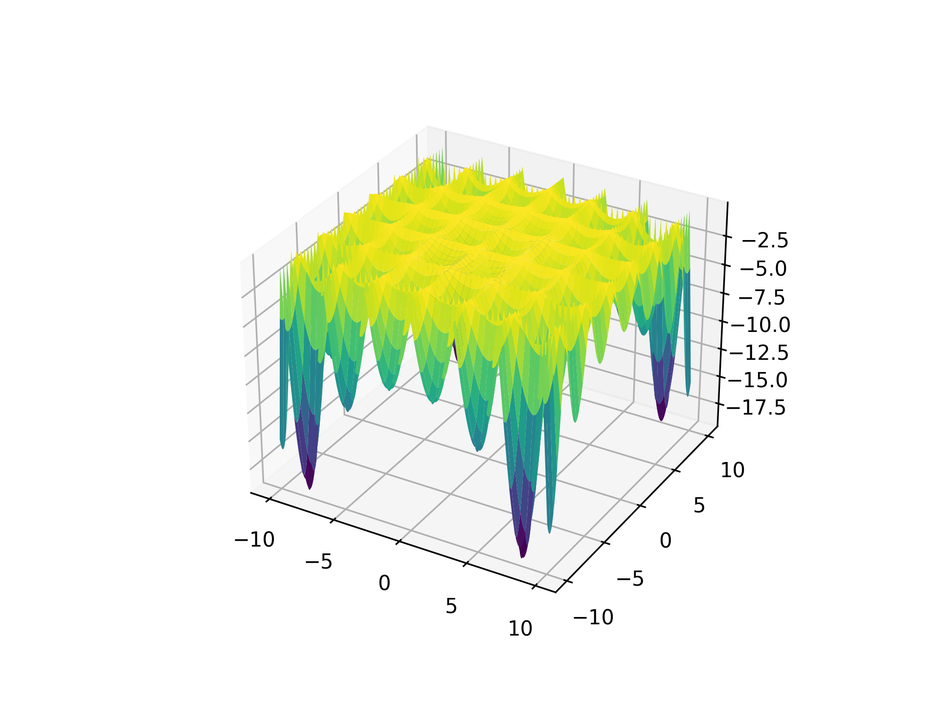 |
Langermann Function
Langermann function.
The Langermann function is a multi-dimensional function with many unevenly distributed local minima.
Examples:
>>> import matplotlib.pyplot as plt
>>> import numpy as np
>>> from umf.functions.optimization.many_local_minima import LangermannFunction
>>> x = np.linspace(0, 10, 1000)
>>> y = np.linspace(0, 10, 1000)
>>> X, Y = np.meshgrid(x, y)
>>> Z = LangermannFunction(X, Y).__eval__
>>> fig = plt.figure()
>>> ax = fig.add_subplot(111, projection="3d")
>>> _ = ax.plot_surface(X, Y, Z, cmap="viridis")
>>> plt.savefig("langermann.png", dpi=300, transparent=True)
Notes
The Langermann function is defined as:
with the constants :math:c_i and the :math:a_{ij} given by:
Reference: Original implementation can be found here.
Parameters:
| Name | Type | Description | Default |
|---|---|---|---|
*x | UniversalArray | Input data, which has to be two dimensional. | () |
A | UniversalArray | Matrix of constants :math: | None |
c | UniversalArray | Vector of constants :math: | None |
m | int | Number of local minima. Defaults to 5. | 5 |
Source code in src/umf/functions/optimization/many_local_minima.py
class LangermannFunction(OptFunction):
    r"""Langermann function.

    The Langermann function is a multi-dimensional function with many unevenly
    distributed local minima.

    Examples:
        >>> import matplotlib.pyplot as plt
        >>> import numpy as np
        >>> from umf.functions.optimization.many_local_minima import LangermannFunction
        >>> x = np.linspace(0, 10, 1000)
        >>> y = np.linspace(0, 10, 1000)
        >>> X, Y = np.meshgrid(x, y)
        >>> Z = LangermannFunction(X, Y).__eval__
        >>> fig = plt.figure()
        >>> ax = fig.add_subplot(111, projection="3d")
        >>> _ = ax.plot_surface(X, Y, Z, cmap="viridis")
        >>> plt.savefig("langermann.png", dpi=300, transparent=True)

    Notes:
        The Langermann function is defined as:

        $$
            f(x) = \sum_{i=1}^{5} c_i \exp \left( -\frac{1}{\pi} \sum_{j=1}^{2}
            (x_j - a_{ij})^2 \right) \cos \left( \pi
            \sum_{j=1}^{2} (x_j - a_{ij})^2 \right)
        $$

        with the constants :math:`c_i` and the :math:`a_{ij}` given by:

        $$
            c_i = \left\{ 1, 2, 5, 2, 3 \right\}, \quad a_{ij} =
            \left\{ 3, 5, 2, 1, 7 \right\}
        $$

        > Reference: Original implementation can be found
        > [here](https://www.sfu.ca/~ssurjano/langer.html).

    Args:
        *x (UniversalArray): Input data, which has to be two dimensional.
        A (UniversalArray, optional): Matrix of constants :math:`a_{ij}`. The numbers
            of rows has to be equal to the number of input data, respectively,
            dimensions. Defaults to :math:`a_{ij} = \left\{ 3, 5, 2, 1, 7 \right\}`.
        c (UniversalArray, optional): Vector of constants :math:`c_i`. Defaults to
            :math:`c_i = \left\{ 1, 2, 5, 2, 3 \right\}`.
        m (int, optional): Number of local minima. Defaults to 5.
    """

    def __init__(
        self,
        *x: UniversalArray,
        A: UniversalArray = None,
        c: UniversalArray = None,
        m: int = 5,
    ) -> None:
        """Initialize the function."""
        super().__init__(*x)

        if A is None:
            A = np.array([[3, 5, 2, 1, 7], [5, 2, 1, 4, 9]], dtype=float)  # noqa: N806

        if c is None:
            c = np.array([1, 2, 5, 2, 3], dtype=float)

        if len(x) != A.shape[0]:
            msg = "Dimension of x must match number of rows in A."
            raise ValueError(msg)

        if len(A.shape) != __2d__:
            msg = (
                "A must be two dimensional array. In case of one input the  "
                "array must lool like 'np.array([[...]])'. "
            )
            raise ValueError(
                msg,
            )
        if A.shape[1] != m:
            raise MatchLengthError(_object="A", _target="m")

        if len(c) != m:
            raise MatchLengthError(_object="C", _target="m")

        if len(c.shape) != __1d__:
            msg = "c must be one dimensional array."
            raise ValueError(msg)

        self.a_matrix = A
        self._c = c
        self._m = m

    @property
    def __eval__(self) -> UniversalArray:
        """Evaluate Langermann function at x.

        Returns:
            UniversalArray: Function values as numpy arrays.
        """
        outer_sum = np.zeros_like(self._x[0])
        for i in range(self._m):
            inner_sum = np.zeros_like(self._x[0])
            for j, _x in enumerate(self._x):
                inner_sum += (_x - self.a_matrix[j, i]) ** 2
            outer_sum += (
                self._c[i] * np.exp(-inner_sum / np.pi) * np.cos(np.pi * inner_sum)
            )
        return outer_sum

    @property
    def __minima__(self) -> MinimaAPI:
        """Return the minima of the function.

        Returns:
            MinimaAPI: MinimaAPI object containing the minima of the function.
        """
        return MinimaAPI(
            f_x=0.0,
            x=tuple(
                np.array([self.a_matrix[0, i], self.a_matrix[1, i]])
                for i in range(self._m)
            ),
        )
__eval__ property ¶Evaluate Langermann function at x.
Returns:
| Name | Type | Description |
|---|---|---|
UniversalArray | UniversalArray | Function values as numpy arrays. |
__minima__ property ¶Return the minima of the function.
Returns:
| Name | Type | Description |
|---|---|---|
MinimaAPI | MinimaAPI | MinimaAPI object containing the minima of the function. |
__init__(*x, A=None, c=None, m=5) ¶Initialize the function.
Source code in src/umf/functions/optimization/many_local_minima.py
def __init__(
    self,
    *x: UniversalArray,
    A: UniversalArray = None,
    c: UniversalArray = None,
    m: int = 5,
) -> None:
    """Initialize the function."""
    super().__init__(*x)

    if A is None:
        A = np.array([[3, 5, 2, 1, 7], [5, 2, 1, 4, 9]], dtype=float)  # noqa: N806

    if c is None:
        c = np.array([1, 2, 5, 2, 3], dtype=float)

    if len(x) != A.shape[0]:
        msg = "Dimension of x must match number of rows in A."
        raise ValueError(msg)

    if len(A.shape) != __2d__:
        msg = (
            "A must be two dimensional array. In case of one input the  "
            "array must lool like 'np.array([[...]])'. "
        )
        raise ValueError(
            msg,
        )
    if A.shape[1] != m:
        raise MatchLengthError(_object="A", _target="m")

    if len(c) != m:
        raise MatchLengthError(_object="C", _target="m")

    if len(c.shape) != __1d__:
        msg = "c must be one dimensional array."
        raise ValueError(msg)

    self.a_matrix = A
    self._c = c
    self._m = m
 |
Levy Function
Levy function.
The Levy function is a multi-dimensional function with many local and harmonic distributed minima.
Examples:
>>> import matplotlib.pyplot as plt
>>> import numpy as np
>>> from umf.functions.optimization.many_local_minima import LevyFunction
>>> x = np.linspace(-10, 10, 1000)
>>> y = np.linspace(-10, 10, 1000)
>>> X, Y = np.meshgrid(x, y)
>>> Z = LevyFunction(X, Y).__eval__
>>> fig = plt.figure()
>>> ax = fig.add_subplot(111, projection="3d")
>>> _ = ax.plot_surface(X, Y, Z, cmap="viridis")
>>> plt.savefig("LevyFunction.png", dpi=300, transparent=True)
Notes
The Levy function is defined as:
with the :math:w_i given by:
Reference: Original implementation can be found here.
Parameters:
| Name | Type | Description | Default |
|---|---|---|---|
*x | UniversalArray | Input data, which has to be two dimensional. | () |
Source code in src/umf/functions/optimization/many_local_minima.py
class LevyFunction(OptFunction):
    r"""Levy function.

    The Levy function is a multi-dimensional function with many local and harmonic
    distributed minima.

    Examples:
        >>> import matplotlib.pyplot as plt
        >>> import numpy as np
        >>> from umf.functions.optimization.many_local_minima import LevyFunction
        >>> x = np.linspace(-10, 10, 1000)
        >>> y = np.linspace(-10, 10, 1000)
        >>> X, Y = np.meshgrid(x, y)
        >>> Z = LevyFunction(X, Y).__eval__
        >>> fig = plt.figure()
        >>> ax = fig.add_subplot(111, projection="3d")
        >>> _ = ax.plot_surface(X, Y, Z, cmap="viridis")
        >>> plt.savefig("LevyFunction.png", dpi=300, transparent=True)

    Notes:
        The Levy function is defined as:

        $$
            f(x) = \sin^2( \pi w_1 ) + \sum_{i=1}^{d-1} \left( w_i - 1 \right)^2 \left[
            1 + 10 \sin^2( \pi w_i + 1 ) \right]
            + \left( w_d - 1 \right)^2 \left[
            1 + \sin^2( 2 \pi w_d ) \right]
        $$

        with the :math:`w_i` given by:

        $$
            w_i = 1 + \frac{1}{4} (x_i - 1) \quad \forall i \in
            \left\{ 1, \dots, d \right\}
        $$

        > Reference: Original implementation can be found
        > [here](https://www.sfu.ca/~ssurjano/levy.html).

    Args:
        *x (UniversalArray): Input data, which has to be two dimensional.
    """

    @property
    def __eval__(self) -> UniversalArray:
        """Evaluate Levy function at x.

        Returns:
            UniversalArray: Function values as numpy arrays.
        """
        sum_ = np.zeros_like(self._x[0])

        term_1 = np.sin(np.pi * (1 + (1 / 4) * (self._x[0] - 1))) ** 2

        if len(self._x) == 1:
            return term_1

        for i in range(1, len(self._x) - 1):
            term_2 = (1 + (1 / 4) * (self._x[i] - 1)) ** 2
            term_3 = 1 + 10 * np.sin(np.pi * (1 + (1 / 4) * (self._x[i] - 1)) + 1) ** 2
            sum_ += term_2 * term_3

        term_4 = (1 + (1 / 4) * (self._x[-1] - 1)) ** 2
        term_5 = (1 + np.sin(2 * np.pi * (1 + (1 / 4) * (self._x[-1] - 1)))) ** 2
        sum_ += term_4 * term_5
        return term_1 + sum_

    @property
    def __minima__(self) -> MinimaAPI:
        """Return the minima of the function.

        Returns:
            MinimaAPI: MinimaAPI object containing the minima of the function.
        """
        return MinimaAPI(
            f_x=0.0,
            x=tuple(np.array([1.0]) for _ in range(len(self._x))),
        )
__eval__ property ¶Evaluate Levy function at x.
Returns:
| Name | Type | Description |
|---|---|---|
UniversalArray | UniversalArray | Function values as numpy arrays. |
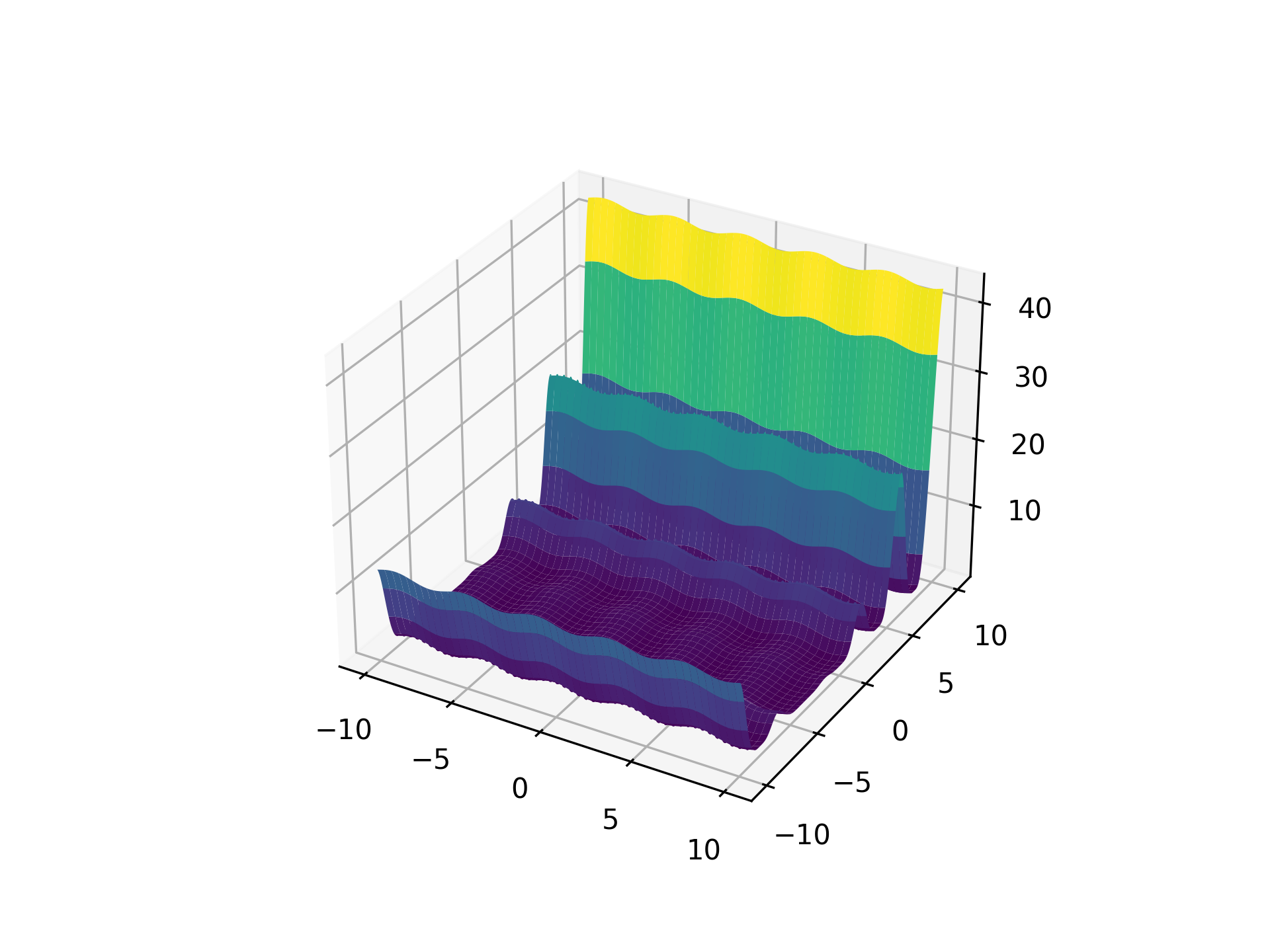 |
Levy Function N. 13
Levy N. 13 function.
The Levy N. 13 function is a two-dimensional function with many local and harmonic and parabolic distributed minima.
Examples:
>>> import matplotlib.pyplot as plt
>>> import numpy as np
>>> from umf.functions.optimization.many_local_minima import LevyN13Function
>>> x = np.linspace(-10, 10, 1000)
>>> y = np.linspace(-10, 10, 1000)
>>> X, Y = np.meshgrid(x, y)
>>> Z = LevyN13Function(X, Y).__eval__
>>> fig = plt.figure()
>>> ax = fig.add_subplot(111, projection="3d")
>>> _ = ax.plot_surface(X, Y, Z, cmap="viridis")
>>> plt.savefig("LevyN13Function.png", dpi=300, transparent=True)
Notes
The Levy N. 13 function is defined as:
Reference: Original implementation can be found here.
Parameters:
| Name | Type | Description | Default |
|---|---|---|---|
*x | UniversalArray | Input data, which has to be two dimensional. | () |
Source code in src/umf/functions/optimization/many_local_minima.py
class LevyN13Function(OptFunction):
    r"""Levy N. 13 function.

    The Levy N. 13 function is a two-dimensional function with many local and harmonic
    and parabolic distributed minima.

    Examples:
        >>> import matplotlib.pyplot as plt
        >>> import numpy as np
        >>> from umf.functions.optimization.many_local_minima import LevyN13Function
        >>> x = np.linspace(-10, 10, 1000)
        >>> y = np.linspace(-10, 10, 1000)
        >>> X, Y = np.meshgrid(x, y)
        >>> Z = LevyN13Function(X, Y).__eval__
        >>> fig = plt.figure()
        >>> ax = fig.add_subplot(111, projection="3d")
        >>> _ = ax.plot_surface(X, Y, Z, cmap="viridis")
        >>> plt.savefig("LevyN13Function.png", dpi=300, transparent=True)

    Notes:
        The Levy N. 13 function is defined as:

        $$
            f(x) = \sin^2( 3 \pi x_1 ) + \left( x_1 - 1 \right)^2 \left[ 1
            + \sin^2( 3 \pi x_2) \right] + \left( x_2 - 1 \right)^2 \left[ 1
            + \sin^2( 2 \pi x_2 ) \right]
        $$

        > Reference: Original implementation can be found
        > [here](https://www.sfu.ca/~ssurjano/levy13.html).

    Args:
        *x (UniversalArray): Input data, which has to be two dimensional.
    """

    def __init__(self, *x: UniversalArray) -> None:
        """Initialize the function."""
        if len(x) != __2d__:
            raise OutOfDimensionError(
                function_name="Levy N. 13",
                dimension=__2d__,
            )
        super().__init__(*x)

    @property
    def __eval__(self) -> UniversalArray:
        """Evaluate Levy N. 13 function at x.

        Returns:
            UniversalArray: Function values as numpy arrays.
        """
        x_1 = self._x[0]
        x_2 = self._x[1]

        term_1 = np.sin(3 * np.pi * x_1) ** 2
        term_2 = (x_1 - 1) ** 2
        term_3 = 1 + np.sin(3 * np.pi * x_2) ** 2
        term_4 = (x_2 - 1) ** 2
        term_5 = 1 + np.sin(2 * np.pi * x_2) ** 2
        return term_1 + term_2 * term_3 + term_4 * term_5

    @property
    def __minima__(self) -> MinimaAPI:
        """Return the minima of the function.

        Returns:
            MinimaAPI: MinimaAPI object containing the minima of the function.
        """
        return MinimaAPI(
            f_x=0.0,
            x=(1.0, 1.0),
        )
__eval__ property ¶Evaluate Levy N. 13 function at x.
Returns:
| Name | Type | Description |
|---|---|---|
UniversalArray | UniversalArray | Function values as numpy arrays. |
__minima__ property ¶Return the minima of the function.
Returns:
| Name | Type | Description |
|---|---|---|
MinimaAPI | MinimaAPI | MinimaAPI object containing the minima of the function. |
__init__(*x) ¶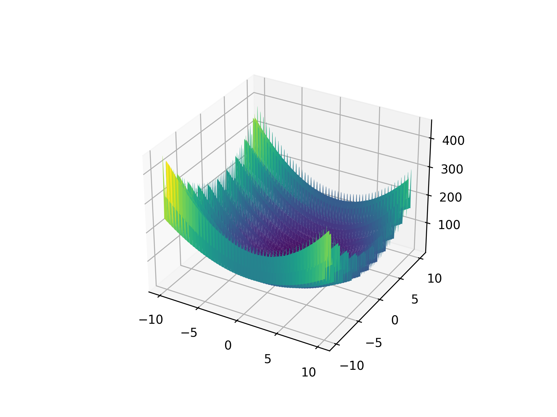 |
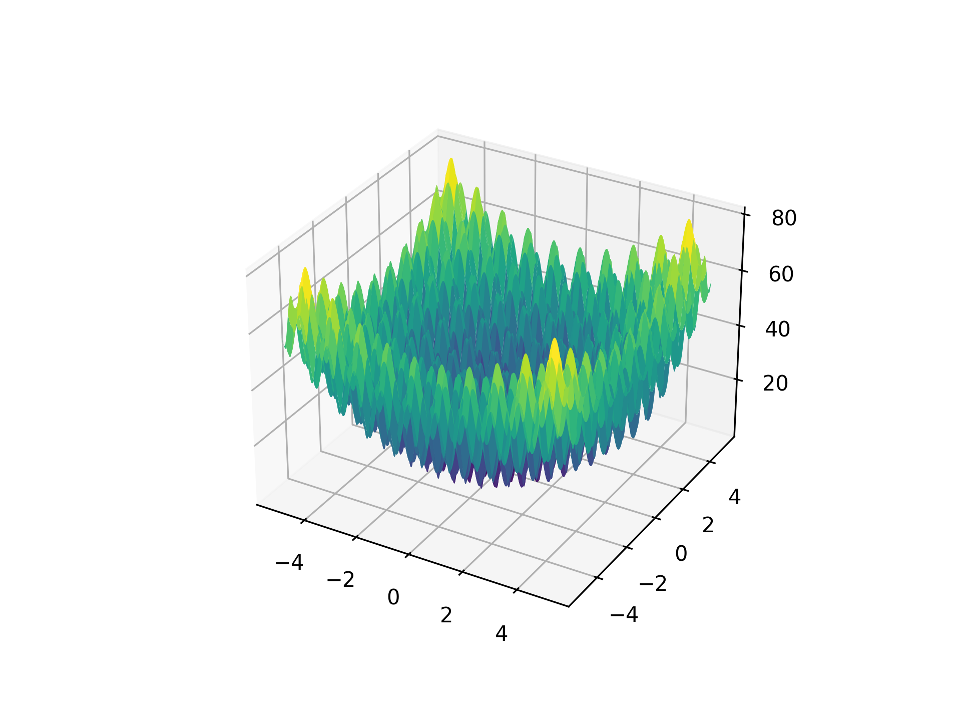
Rastrigin Function
Rastrigin function.
The Rastrigin function is a multi-dimensional function with many local and harmonic and parabolic distributed minima.
Examples:
>>> import matplotlib.pyplot as plt
>>> import numpy as np
>>> from umf.functions.optimization.many_local_minima import RastriginFunction
>>> x = np.linspace(-5.12, 5.12, 1000)
>>> y = np.linspace(-5.12, 5.12, 1000)
>>> X, Y = np.meshgrid(x, y)
>>> Z = RastriginFunction(X, Y).__eval__
>>> fig = plt.figure()
>>> ax = fig.add_subplot(111, projection="3d")
>>> _ = ax.plot_surface(X, Y, Z, cmap="viridis")
>>> plt.savefig("RastriginFunction.png", dpi=300, transparent=True)
Notes
The Rastrigin function is defined as:
Reference: Original implementation can be found here.
Parameters:
| Name | Type | Description | Default |
|---|---|---|---|
*x | UniversalArray | Input data, which has to be two dimensional. | () |
Source code in src/umf/functions/optimization/many_local_minima.py
class RastriginFunction(OptFunction):
    r"""Rastrigin function.

    The Rastrigin function is a multi-dimensional function with many local and harmonic
    and parabolic distributed minima.

    Examples:
        >>> import matplotlib.pyplot as plt
        >>> import numpy as np
        >>> from umf.functions.optimization.many_local_minima import RastriginFunction
        >>> x = np.linspace(-5.12, 5.12, 1000)
        >>> y = np.linspace(-5.12, 5.12, 1000)
        >>> X, Y = np.meshgrid(x, y)
        >>> Z = RastriginFunction(X, Y).__eval__
        >>> fig = plt.figure()
        >>> ax = fig.add_subplot(111, projection="3d")
        >>> _ = ax.plot_surface(X, Y, Z, cmap="viridis")
        >>> plt.savefig("RastriginFunction.png", dpi=300, transparent=True)

    Notes:
        The Rastrigin function is defined as:

        $$
            f(x) = 10 n + \sum_{i=1}^n \left[ x_i^2 - 10 \cos(2 \pi x_i) \right]
        $$

        > Reference: Original implementation can be found
        > [here](https://www.sfu.ca/~ssurjano/rastr.html).

    Args:
        *x (UniversalArray): Input data, which has to be two dimensional.
    """

    @property
    def __eval__(self) -> UniversalArray:
        """Evaluate Rastrigin function at x.

        Returns:
            UniversalArray: Function values as numpy arrays.
        """
        sum_ = np.zeros_like(self._x[0])
        for x_i in self._x:
            sum_ += x_i**2 - 10 * np.cos(2 * np.pi * x_i)
        return 10 * len(self._x) + sum_

    @property
    def __minima__(self) -> MinimaAPI:
        """Return the minima of the function.

        Returns:
            MinimaAPI: MinimaAPI object containing the minima of the function.
        """
        return MinimaAPI(
            f_x=0.0,
            x=tuple(np.array([0.0]) for _ in range(len(self._x))),
        )
__eval__ property ¶Evaluate Rastrigin function at x.
Returns:
| Name | Type | Description |
|---|---|---|
UniversalArray | UniversalArray | Function values as numpy arrays. |
 |
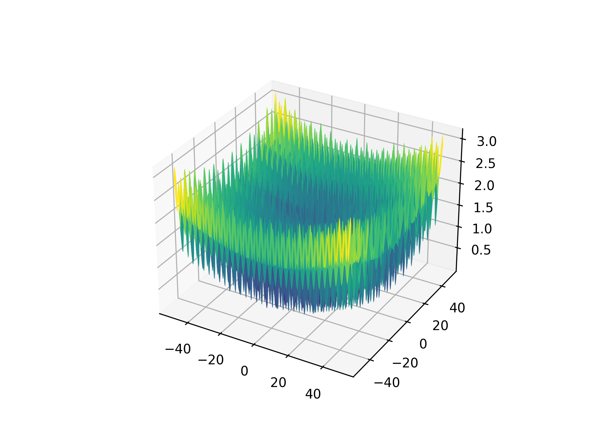
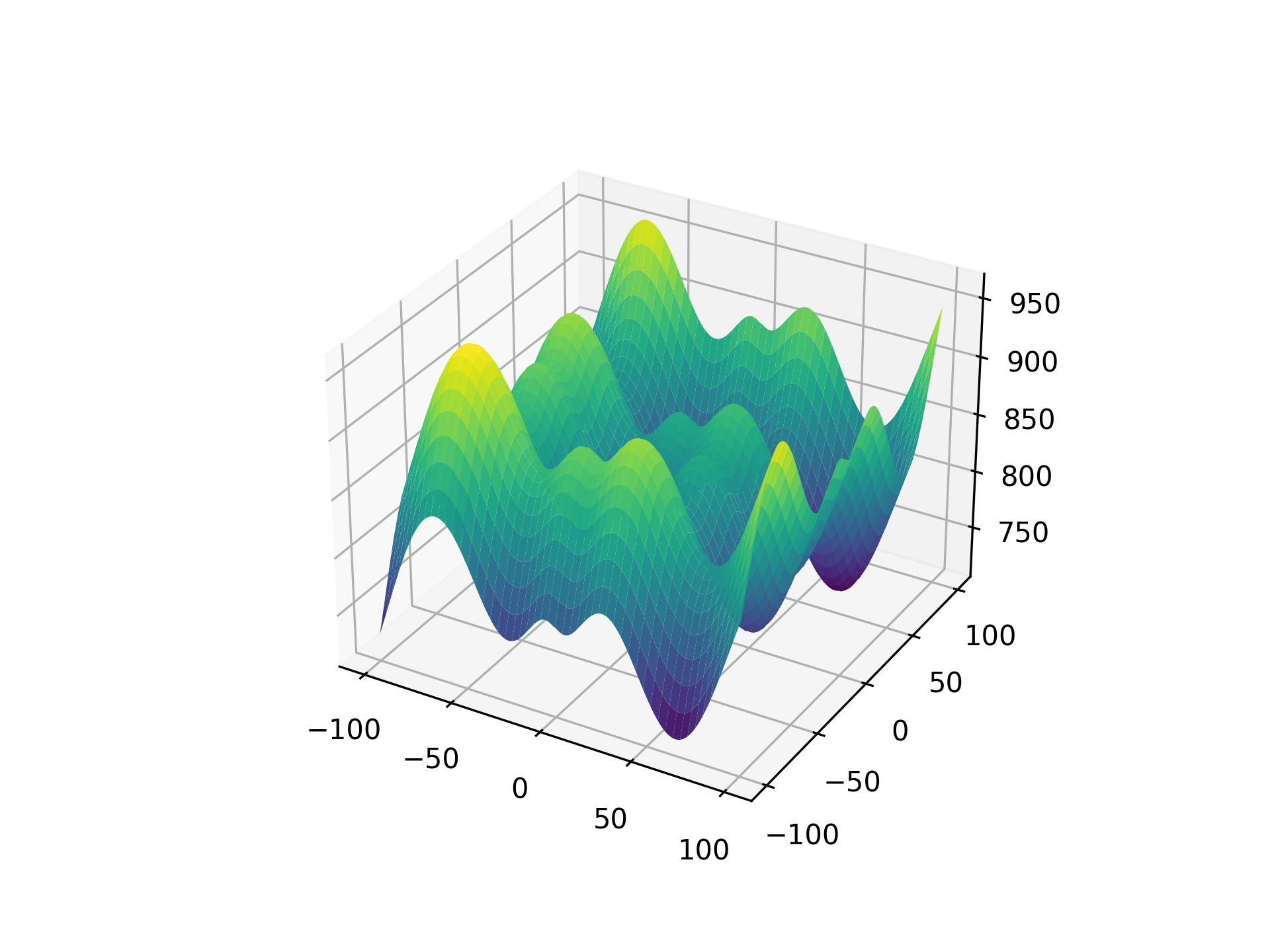
Schaffer Function N. 2
Schaffer N. 2 function.
The Schaffer N. 2 function is a two-dimensional function with a single global minimum and radial distributed local minima.
Examples:
>>> import matplotlib.pyplot as plt
>>> import numpy as np
>>> from umf.functions.optimization.many_local_minima import SchafferN2Function
>>> x = np.linspace(-100, 100, 1000)
>>> y = np.linspace(-100, 100, 1000)
>>> X, Y = np.meshgrid(x, y)
>>> Z = SchafferN2Function(X, Y).__eval__
>>> fig = plt.figure()
>>> ax = fig.add_subplot(111, projection="3d")
>>> _ = ax.plot_surface(X, Y, Z, cmap="viridis")
>>> plt.savefig("SchafferN2Function.png", dpi=300, transparent=True)
Notes
The Schaffer N. 2 function is defined as:
Reference: Original implementation can be found here.
Parameters:
| Name | Type | Description | Default |
|---|---|---|---|
*x | UniversalArray | Input data, which has to be two dimensional. | () |
Source code in src/umf/functions/optimization/many_local_minima.py
class SchafferN2Function(OptFunction):
    r"""Schaffer N. 2 function.

    The Schaffer N. 2 function is a two-dimensional function with a
    single global minimum and radial distributed local minima.

    Examples:
        >>> import matplotlib.pyplot as plt
        >>> import numpy as np
        >>> from umf.functions.optimization.many_local_minima import SchafferN2Function
        >>> x = np.linspace(-100, 100, 1000)
        >>> y = np.linspace(-100, 100, 1000)
        >>> X, Y = np.meshgrid(x, y)
        >>> Z = SchafferN2Function(X, Y).__eval__
        >>> fig = plt.figure()
        >>> ax = fig.add_subplot(111, projection="3d")
        >>> _ = ax.plot_surface(X, Y, Z, cmap="viridis")
        >>> plt.savefig("SchafferN2Function.png", dpi=300, transparent=True)

    Notes:
        The Schaffer N. 2 function is defined as:

        $$
            f(x) = \frac{1}{2} + \frac{ \sin^2 \left( \left| x_1^2 + x_2^2 \right|
            \right) - 0.5 }{ \left( 1 + 0.001 \left( x_1^2 + x_2^2 \right) \right)^2 }
        $$

        > Reference: Original implementation can be found
        > [here](https://www.sfu.ca/~ssurjano/schaffer2.html).

    Args:
        *x (UniversalArray): Input data, which has to be two dimensional.
    """

    def __init__(self, *x: UniversalArray) -> None:
        """Initialize the function."""
        if len(x) != __2d__:
            raise OutOfDimensionError(
                function_name="Schaffer N. 2",
                dimension=__2d__,
            )
        super().__init__(*x)

    @property
    def __eval__(self) -> UniversalArray:
        """Evaluate Schaffer N. 2 function at x.

        Returns:
            UniversalArray: Function values as numpy arrays.
        """
        x_1 = self._x[0]
        x_2 = self._x[1]
        return (
            0.5
            + (np.sin(np.abs(x_1**2 + x_2**2)) ** 2 - 0.5)
            / (1 + 0.001 * (x_1**2 + x_2**2)) ** 2
        )

    @property
    def __minima__(self) -> MinimaAPI:
        """Return the minima of the function.

        Returns:
            MinimaAPI: MinimaAPI object containing the minima of the function.
        """
        return MinimaAPI(
            f_x=0.0,
            x=(0.0, 0.0),
        )
__eval__ property ¶Evaluate Schaffer N. 2 function at x.
Returns:
| Name | Type | Description |
|---|---|---|
UniversalArray | UniversalArray | Function values as numpy arrays. |
__minima__ property ¶Return the minima of the function.
Returns:
| Name | Type | Description |
|---|---|---|
MinimaAPI | MinimaAPI | MinimaAPI object containing the minima of the function. |
__init__(*x) ¶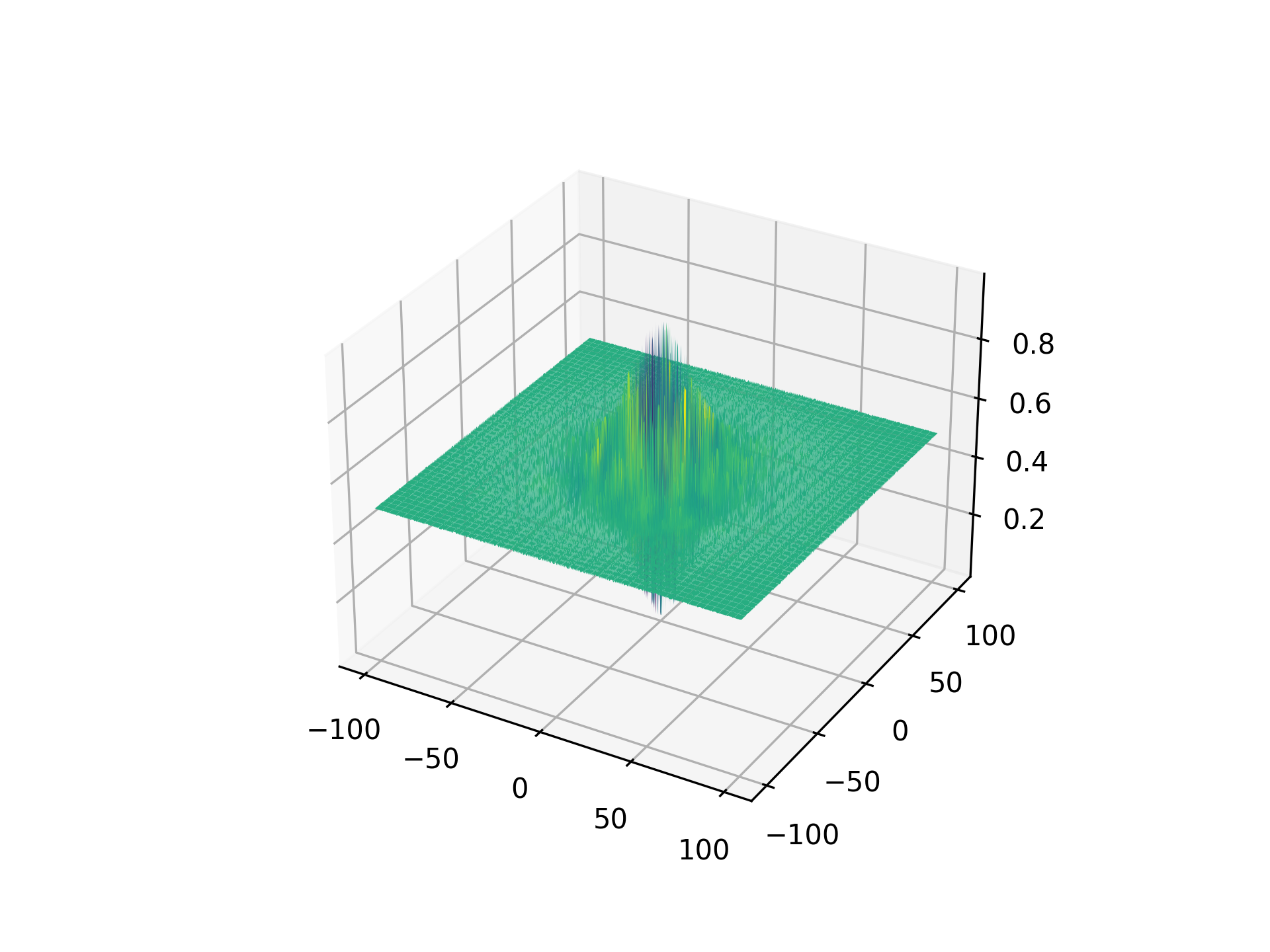 |
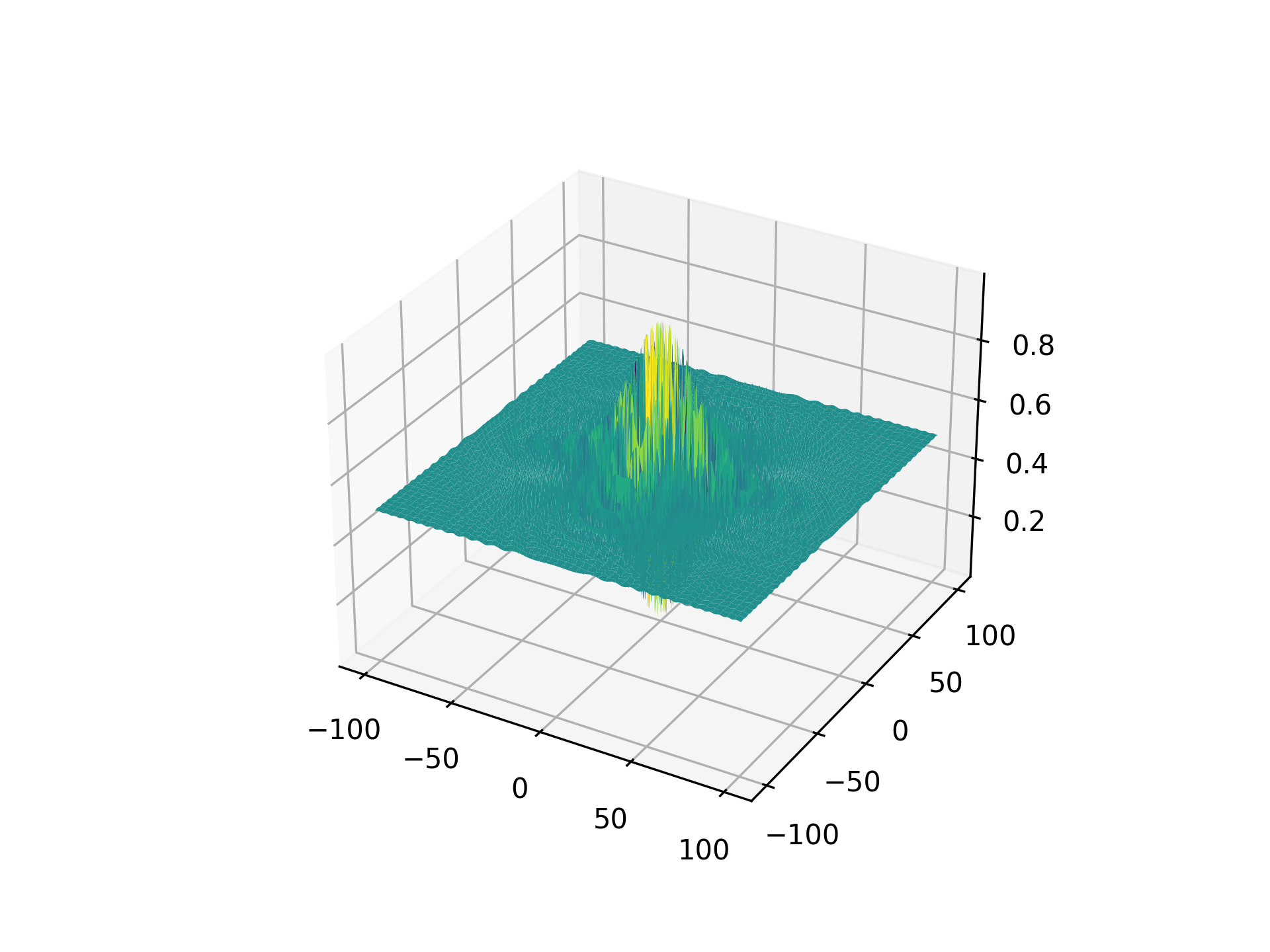
Schaffer Function N. 4
Schaffer N. 4 function.
The Schaffer N. 4 function is a two-dimensional function with a single global minimum and radial distributed local minima.
Examples:
>>> import matplotlib.pyplot as plt
>>> import numpy as np
>>> from umf.functions.optimization.many_local_minima import SchafferN4Function
>>> x = np.linspace(-100, 100, 1000)
>>> y = np.linspace(-100, 100, 1000)
>>> X, Y = np.meshgrid(x, y)
>>> Z = SchafferN4Function(X, Y).__eval__
>>> fig = plt.figure()
>>> ax = fig.add_subplot(111, projection="3d")
>>> _ = ax.plot_surface(X, Y, Z, cmap="viridis")
>>> plt.savefig("SchafferN4Function.png", dpi=300, transparent=True)
Notes
The Schaffer N. 4 function is defined as:
Reference: Original implementation can be found here.
Parameters:
| Name | Type | Description | Default |
|---|---|---|---|
*x | UniversalArray | Input data, which has to be two dimensional. | () |
Source code in src/umf/functions/optimization/many_local_minima.py
class SchafferN4Function(OptFunction):
    r"""Schaffer N. 4 function.

    The Schaffer N. 4 function is a two-dimensional function with a
    single global minimum and radial distributed local minima.

    Examples:
        >>> import matplotlib.pyplot as plt
        >>> import numpy as np
        >>> from umf.functions.optimization.many_local_minima import SchafferN4Function
        >>> x = np.linspace(-100, 100, 1000)
        >>> y = np.linspace(-100, 100, 1000)
        >>> X, Y = np.meshgrid(x, y)
        >>> Z = SchafferN4Function(X, Y).__eval__
        >>> fig = plt.figure()
        >>> ax = fig.add_subplot(111, projection="3d")
        >>> _ = ax.plot_surface(X, Y, Z, cmap="viridis")
        >>> plt.savefig("SchafferN4Function.png", dpi=300, transparent=True)

    Notes:
        The Schaffer N. 4 function is defined as:

        $$
            f(x) = 0.5 + \frac{ \sin^2 \left( \sqrt{ x_1^2 + x_2^2 } \right) - 0.5 }
            { \left( 1 + 0.001 \left( x_1^2 + x_2^2 \right) \right)^2 }
        $$

        > Reference: Original implementation can be found
        > [here](https://www.sfu.ca/~ssurjano/schaffer4.html).

    Args:
        *x (UniversalArray): Input data, which has to be two dimensional.
    """

    def __init__(self, *x: UniversalArray) -> None:
        """Initialize the function."""
        if len(x) != __2d__:
            raise OutOfDimensionError(
                function_name="Schaffer N. 4",
                dimension=__2d__,
            )
        super().__init__(*x)

    @property
    def __eval__(self) -> UniversalArray:
        """Evaluate Schaffer N. 4 function at x.

        Returns:
            UniversalArray: Function values as numpy arrays.
        """
        x_1 = self._x[0]
        x_2 = self._x[1]
        return (
            0.5
            + (np.sin(np.sqrt(x_1**2 + x_2**2)) ** 2 - 0.5)
            / (1 + 0.001 * (x_1**2 + x_2**2)) ** 2
        )

    @property
    def __minima__(self) -> MinimaAPI:
        """Return the minima of the function."""
        return MinimaAPI(
            f_x=0.0,
            x=(0.0, 0.0),
        )
 |
Schwefel Function
Schwefel function.
The Schwefel function is a multi-dimensional function with a single global minimum.
Examples:
>>> import matplotlib.pyplot as plt
>>> import numpy as np
>>> from umf.functions.optimization.many_local_minima import SchwefelFunction
>>> x = np.linspace(-100, 100, 1000)
>>> y = np.linspace(-100, 100, 1000)
>>> X, Y = np.meshgrid(x, y)
>>> Z = SchwefelFunction(X, Y).__eval__
>>> fig = plt.figure()
>>> ax = fig.add_subplot(111, projection="3d")
>>> _ = ax.plot_surface(X, Y, Z, cmap="viridis")
>>> plt.savefig("SchwefelFunction.png", dpi=300, transparent=True)
Notes
The Schwefel function is defined as:
Reference: Original implementation can be found here.
Parameters:
| Name | Type | Description | Default |
|---|---|---|---|
*x | UniversalArray | Input data, which has to be two dimensional. | () |
Source code in src/umf/functions/optimization/many_local_minima.py
class SchwefelFunction(OptFunction):
    r"""Schwefel function.

    The Schwefel function is a multi-dimensional function with a
    single global minimum.

    Examples:
        >>> import matplotlib.pyplot as plt
        >>> import numpy as np
        >>> from umf.functions.optimization.many_local_minima import SchwefelFunction
        >>> x = np.linspace(-100, 100, 1000)
        >>> y = np.linspace(-100, 100, 1000)
        >>> X, Y = np.meshgrid(x, y)
        >>> Z = SchwefelFunction(X, Y).__eval__
        >>> fig = plt.figure()
        >>> ax = fig.add_subplot(111, projection="3d")
        >>> _ = ax.plot_surface(X, Y, Z, cmap="viridis")
        >>> plt.savefig("SchwefelFunction.png", dpi=300, transparent=True)

    Notes:
        The Schwefel function is defined as:

        $$
            f(x) = 418.9829 n - \sum_{i=1}^{n} x_i \sin
            \left( \sqrt{ \left| x_i \right| } \right)
        $$

        > Reference: Original implementation can be found
        > [here](https://www.sfu.ca/~ssurjano/schwef.html).

    Args:
        *x (UniversalArray): Input data, which has to be two dimensional.
    """

    def __init__(self, *x: UniversalArray) -> None:
        """Initialize the function."""
        super().__init__(*x)

    @property
    def __eval__(self) -> UniversalArray:
        """Evaluate Schwefel function at x.

        Returns:
            UniversalArray: Function values as numpy arrays.
        """
        return 418.9829 * len(self._x) - np.sum(
            self._x * np.sin(np.sqrt(np.abs(self._x))),
            axis=0,
        )

    @property
    def __minima__(self) -> MinimaAPI:
        """Return the minima of the function."""
        return MinimaAPI(
            f_x=0.0,
            x=(420.968746, 420.968746),
        )
 |
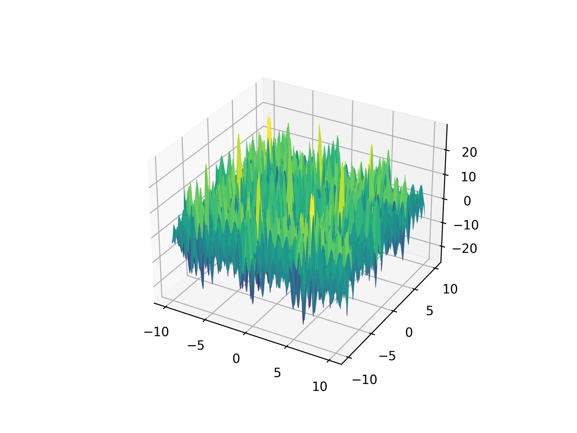
Shubert Function
Shubert function.
The Shubert function is a two-dimensional function with a single global minimum.
Examples:
>>> import matplotlib.pyplot as plt
>>> import numpy as np
>>> from umf.functions.optimization.many_local_minima import ShubertFunction
>>> x = np.linspace(-10, 10, 1000)
>>> y = np.linspace(-10, 10, 1000)
>>> X, Y = np.meshgrid(x, y)
>>> Z = ShubertFunction(X, Y).__eval__
>>> fig = plt.figure()
>>> ax = fig.add_subplot(111, projection="3d")
>>> _ = ax.plot_surface(X, Y, Z, cmap="viridis")
>>> plt.savefig("ShubertFunction.png", dpi=300, transparent=True)
Notes
The Shubert function is defined as:
Reference: Original implementation can be found here.
Parameters:
| Name | Type | Description | Default |
|---|---|---|---|
*x | UniversalArray | Input data, which has to be two dimensional. | () |
Source code in src/umf/functions/optimization/many_local_minima.py
class ShubertFunction(OptFunction):
    r"""Shubert function.

    The Shubert function is a two-dimensional function with a
    single global minimum.

    Examples:
        >>> import matplotlib.pyplot as plt
        >>> import numpy as np
        >>> from umf.functions.optimization.many_local_minima import ShubertFunction
        >>> x = np.linspace(-10, 10, 1000)
        >>> y = np.linspace(-10, 10, 1000)
        >>> X, Y = np.meshgrid(x, y)
        >>> Z = ShubertFunction(X, Y).__eval__
        >>> fig = plt.figure()
        >>> ax = fig.add_subplot(111, projection="3d")
        >>> _ = ax.plot_surface(X, Y, Z, cmap="viridis")
        >>> plt.savefig("ShubertFunction.png", dpi=300, transparent=True)

    Notes:
        The Shubert function is defined as:

        $$
            f(x) = \sum_{i=1}^{5} i \cos \left( \left( i + 1 \right) x_1 + i \right) +
            \sum_{i=1}^{5} i \cos \left( \left( i + 1 \right) x_2 + i \right)
        $$

        > Reference: Original implementation can be found
        > [here](https://www.sfu.ca/~ssurjano/shubert.html).

    Args:
        *x (UniversalArray): Input data, which has to be two dimensional.
    """

    def __init__(self, *x: UniversalArray) -> None:
        """Initialize the function."""
        if len(x) != __2d__:
            raise OutOfDimensionError(
                function_name="Shubert",
                dimension=__2d__,
            )
        super().__init__(*x)

    @property
    def __eval__(self) -> UniversalArray:
        """Evaluate Shubert function at x.

        Returns:
            UniversalArray: Function values as numpy arrays.
        """
        x_1 = self._x[0]
        x_2 = self._x[1]
        return np.sum(
            np.array(
                [
                    i * np.cos((i + 1) * x_1 + i) + i * np.cos((i + 1) * x_2 + i)
                    for i in range(1, 6)
                ],
            ),
            axis=0,
        )

    @property
    def __minima__(self) -> MinimaAPI:
        """Return the minima of the function."""
        return MinimaAPI(f_x=-186.7309, x=(-7.708309818, -0.800371886))
 |
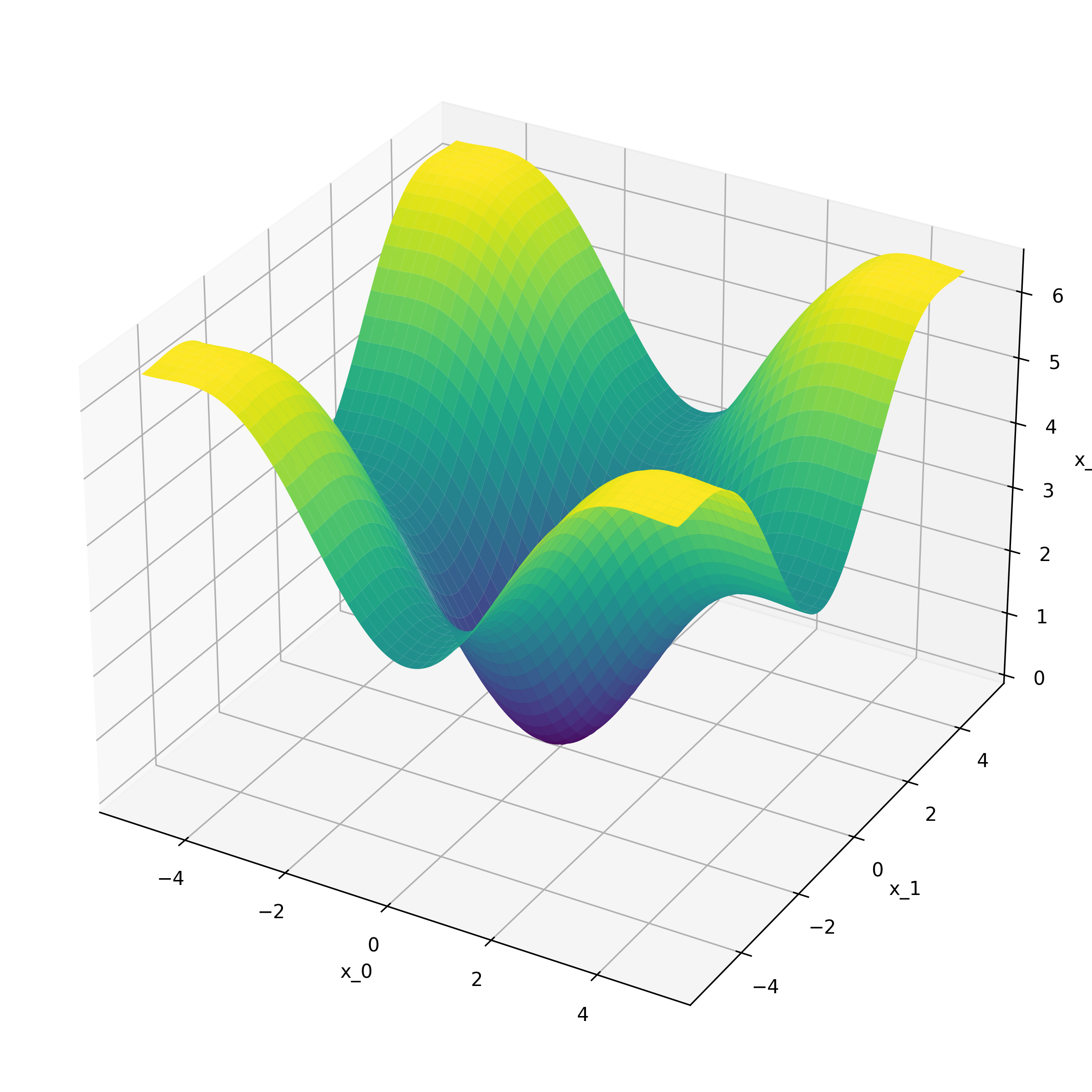
Cosine Mixture Function
Cosine mixture function.
Source code in src/umf/functions/optimization/many_local_minima.py
class CosineMixtureFunction(OptFunction):
    r"""Cosine mixture function."""

    def __init__(self, *x: UniversalArray) -> None:
        """Initialize the cosine mixture function."""
        _validate_two_dimensional(*x, function_name="CosineMixture")
        super().__init__(*x)

    @property
    def __eval__(self) -> UniversalArray:
        """Evaluate the cosine mixture function at x."""
        x_1, x_2 = self._x
        return 0.1 * (x_1**2 + x_2**2) + (1 - np.cos(x_1)) + (1 - np.cos(x_2))

    @property
    def __minima__(self) -> MinimaAPI:
        """Return the minima of the cosine mixture function."""
        return MinimaAPI(f_x=0.0, x=(0.0, 0.0))
 |
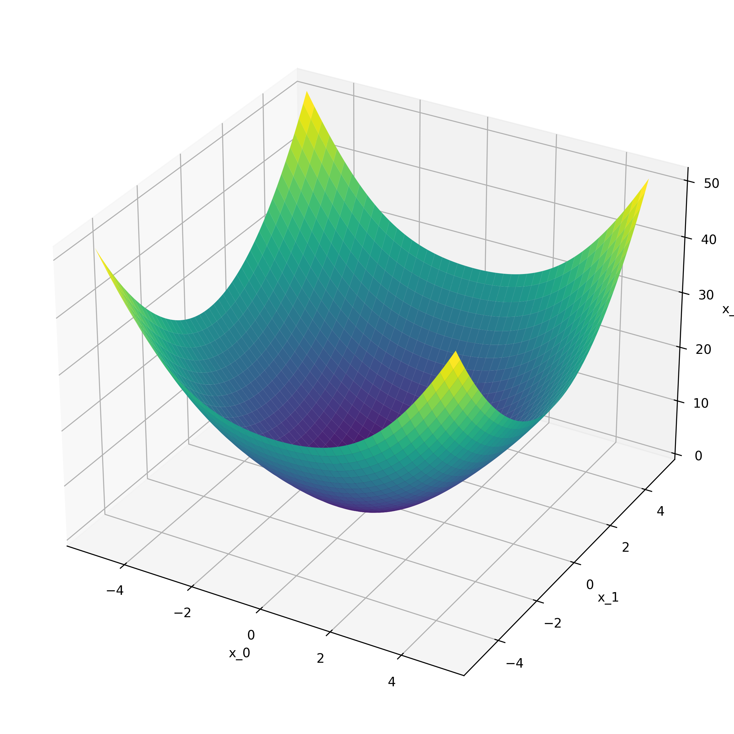
Cosine Product Sphere Function
Cosine-product sphere function.
Source code in src/umf/functions/optimization/many_local_minima.py
class CosineProductSphereFunction(OptFunction):
    r"""Cosine-product sphere function."""

    def __init__(self, *x: UniversalArray) -> None:
        """Initialize the cosine-product sphere function."""
        _validate_three_or_higher(*x, function_name="CosineProductSphere")
        super().__init__(*x)

    @property
    def __eval__(self) -> UniversalArray:
        """Evaluate the cosine-product sphere function at x."""
        indices = np.arange(1, self.dimension + 1)
        cosine_term = np.ones_like(self._x[0])
        for index, axis in zip(indices, self._x, strict=True):
            cosine_term *= np.cos(axis / np.sqrt(index))
        return np.array(sum(axis**2 for axis in self._x) - cosine_term + 1)

    @property
    def __minima__(self) -> MinimaAPI:
        """Return the minima of the cosine-product sphere function."""
        return MinimaAPI(f_x=0.0, x=tuple(0.0 for _ in range(self.dimension)))
 |