2D and 3D Plots

Matplotlib-type Plots¶

Plotting functions using via matplotlib.

Examples:

Python Console Session

>>> from pathlib import Path
>>> import numpy as np
>>> from umf.images.diagrams import ClassicPlot
>>> from umf.meta.plots import GraphSettings
>>> x = np.linspace(-10, 10, 100)
>>> y = np.linspace(-10, 10, 100)
>>> X, Y = np.meshgrid(x, y)
>>> Z = X ** 2 + Y ** 2
>>> plot = ClassicPlot(X, Y, Z, settings=GraphSettings(axis=["x", "y", "z"]))
>>> plot.plot_3d()
>>> ClassicPlot.plot_save(plot.plot_return, Path("ClassicPlot_3d.png"))
>>> plot.plot_contour()
>>> ClassicPlot.plot_save(plot.plot_return, Path("ClassicPlot_contour.png"))
>>> plot.plot_surface()
>>> ClassicPlot.plot_save(plot.plot_return, Path("ClassicPlot_surface.png"))
>>> plot.plot_dashboard()
>>> ClassicPlot.plot_save(plot.plot_return, Path("ClassicPlot_dashboard.png"))
>>> plot.plot_close()

Examples:

Python Console Session

>>> from pathlib import Path
>>> import numpy as np
>>> from umf.images.diagrams import ClassicPlot
>>> from umf.meta.plots import GraphSettings
>>> from umf.meta.plots import GIFSettings
>>> from umf.functions.optimization.special import GoldsteinPriceFunction
>>> # Start with a simple plot
>>> x = np.linspace(-2, 2, 100)
>>> y = np.linspace(-2, 2, 100)
>>> X, Y = np.meshgrid(x, y)
>>> Z = GoldsteinPriceFunction(X, Y).__eval__
>>> plot = ClassicPlot(
...     X,
...     Y,
...     Z,
...     settings=GraphSettings(axis=["x", "y", "z"]),
... )
>>> plot.plot_surface()
>>> # Now only zoom
>>> plot.plot_save_gif(
...     fig=plot.plot_return,
...     ax_fig=plot.ax_return,
...     fname=Path("GoldsteinPriceFunction_zoom.gif"),
...     settings=GIFSettings(),
... )
>>> # Now only rotate
>>> plot.plot_save_gif(
...     fig=plot.plot_return,
...     ax_fig=plot.ax_return,
...     fname=Path("GoldsteinPriceFunction_rotate.gif"),
...     settings=GIFSettings(),
... )
>>> # Now only zoom and rotate
>>> plot.plot_save_gif(
...     fig=plot.plot_return,
...     ax_fig=plot.ax_return,
...     fname=Path("GoldsteinPriceFunction_all.gif"),
...     settings=GIFSettings(),
... )
>>> plot.plot_close()

Examples:

Python Console Session

>>> from pathlib import Path
>>> import numpy as np
>>> from umf.images.diagrams import ClassicPlot
>>> from umf.meta.plots import GraphSettings
>>> from umf.functions.distributions.continuous_semi_infinite_interval import (
...    RayleighDistribution,
... )
>>> x = np.linspace(0, 10, 100)
>>> y_sigma_1 = RayleighDistribution(x, sigma=1).__eval__
>>> y_sigma_2 = RayleighDistribution(x, sigma=2).__eval__
>>> y_sigma_3 = RayleighDistribution(x, sigma=3).__eval__
>>> plot = ClassicPlot(
...     np.array([x, y_sigma_1]),
...     np.array([x, y_sigma_2]),
...     np.array([x, y_sigma_3]),
...     settings=GraphSettings(
...         axis=["x", r"$f(x)$"],
...         title="Rayleigh Distribution",
...     ),
... )
>>> plot.plot_series(label=[r"$\sigma=1$", r"$\sigma=2$", r"$\sigma=3$"])
>>> ClassicPlot.plot_save(plot.plot_return, Path("ClassicPlot_series.png"))

Parameters:

Name	Type	Description	Default
`*x`	`UniversalArray`	Input data, which can be one, two, three, or higher dimensional.	`()`
`settings`	`GraphSettings`	Settings for the graph. Defaults to None.	`None`
`**kwargs`	`dict[str, Any]`	Additional keyword arguments to pass to the plot function.	`{}`

ax_return property ¶

Return the Figure.

plot_return property ¶

Return the plot.

label_settings(*, dim3=False, legend=False) ¶

Set the labels for a 2D or 3D plot.

Parameters:

Name	Type	Description	Default
`ax`	`Figure`	Figure objects to set the labels and title.	required
`dim3`	`bool`	Whether the plot is 3D. Defaults to False.	`False`
`legend`	`bool`	Whether to show the legend. Defaults to False.	`False`

plot_2d(ax=None) ¶

Plot a 2D function.

Parameters:

Name	Type	Description	Default
`ax`	`Figure`	Figure object to plot the data. Defaults to None.	`None`

plot_3d(ax=None) ¶

Plot a 3D function.

Parameters:

Name	Type	Description	Default
`ax`	`Figure`	Figure object to plot the data. Defaults to None.	`None`

plot_close() staticmethod ¶

Close all plots.

plot_contour(ax=None) ¶

Plot a contour plot.

plot_dashboard() ¶

Plot a dashboard.

plot_save(fig, fname, fformat='png', **kwargs) staticmethod ¶

Save the plot.

Parameters:

Name	Type	Description	Default
`fig`	`figure`	The figure to save.	required
`fname`	`Path`	The filename to save the figure to.	required
`fformat`	`str`	The format to save the plot as. Defaults to "png".	`'png'`
`**kwargs`	`dict[str, Any]`	Additional keyword arguments to pass to the save function.	`{}`

plot_save_animation(*, fig, ax_fig, fname, settings, **kwargs) staticmethod ¶

Create and save an animation of a 2D plot with scatter and line elements.

This function generates an animation by progressively revealing data points in both a scatter plot and a line plot, then saves it as an animated file.

Parameters:

Name	Type	Description	Default
`fig`	`Figure`	The matplotlib figure object containing the plot	required
`ax_fig`	`SubFigure`	The axis object containing the plots to animate	required
`fname`	`Path`	Path object specifying where to save the animation file	required
`settings`	`AnimationSettings`	Settings object containing animation parameters like frames, interval, and dpi	required
`**kwargs`	`dict[str, Any]`	Additional keyword arguments passed to animation.save()	`{}`

plot_save_gif(*, fig, ax_fig, fname, settings, **kwargs) staticmethod ¶

Saves the given plot to a file.

Note

For generating GIFs, the a subfunction is used to update the plot for each frame of the animation. This subfunction is defined in the function update.

Parameters:

Name	Type	Description	Default
`fig`	`figure`	The figure to save.	required
`ax_fig`	`Figure`	The figure to save.	required
`fname`	`Path`	The filename to save the figure to.	required
`settings`	`GIFSettings`	The settings for the GIF.	required
`**kwargs`	`dict[str, Any]`	Additional keyword arguments to pass to the save function.	`{}`

plot_series(ax=None, label=None) ¶

Plot a 2D function as a series.

Parameters:

Name	Type	Description	Default
`ax`	`Figure`	Figure object to plot the data. Defaults to None.	`None`
`label`	`list[str \| None]`	The label of each line. Defaults to None.	`None`

plot_show() ¶

Show the plot.

plot_surface(ax=None) ¶

Plot a 3D function.

Types	Matplotlib-type Plots
3D-Plot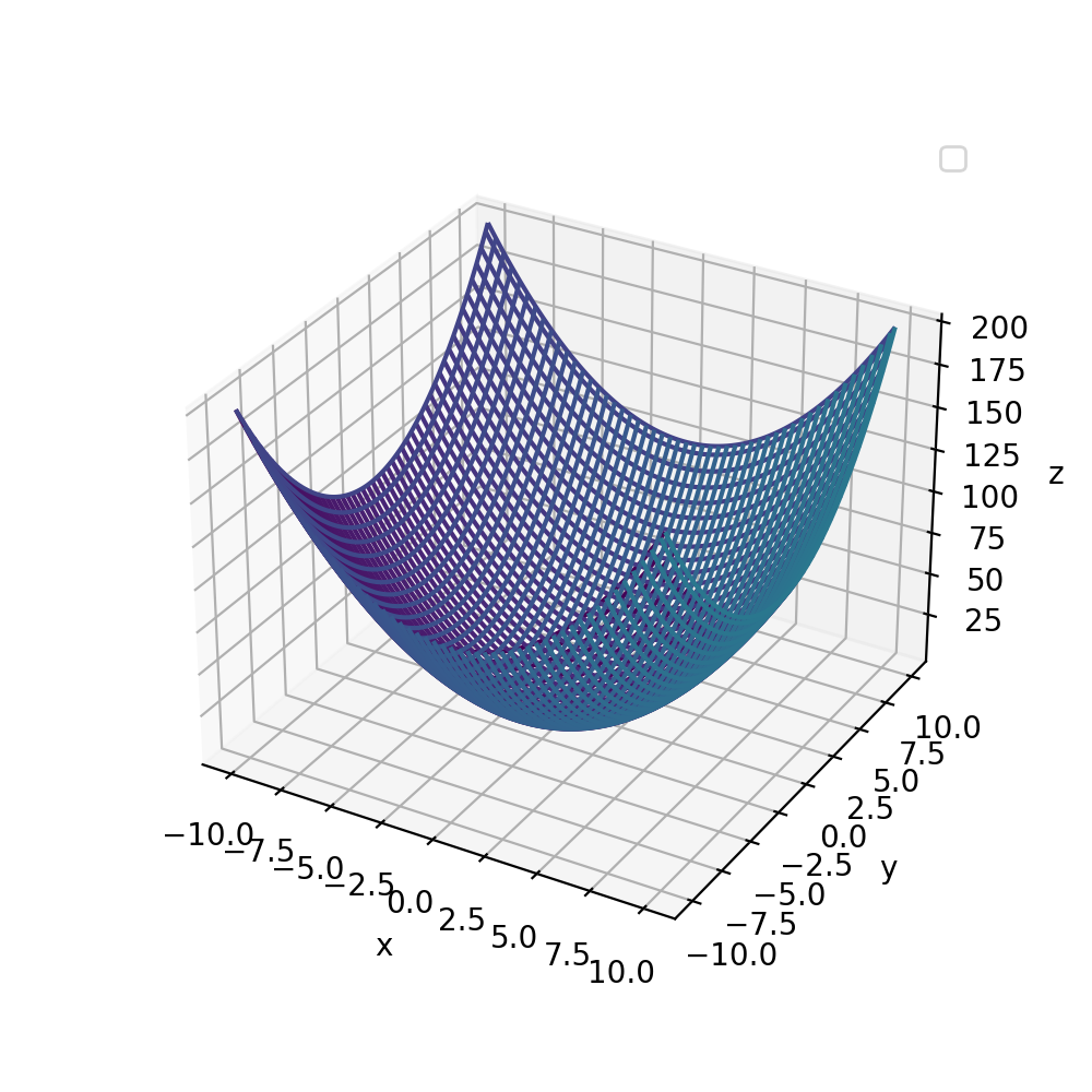
Contour-Plot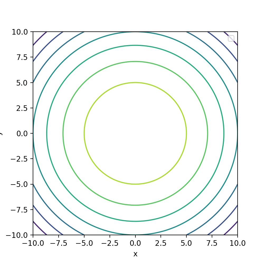
Surface-Plot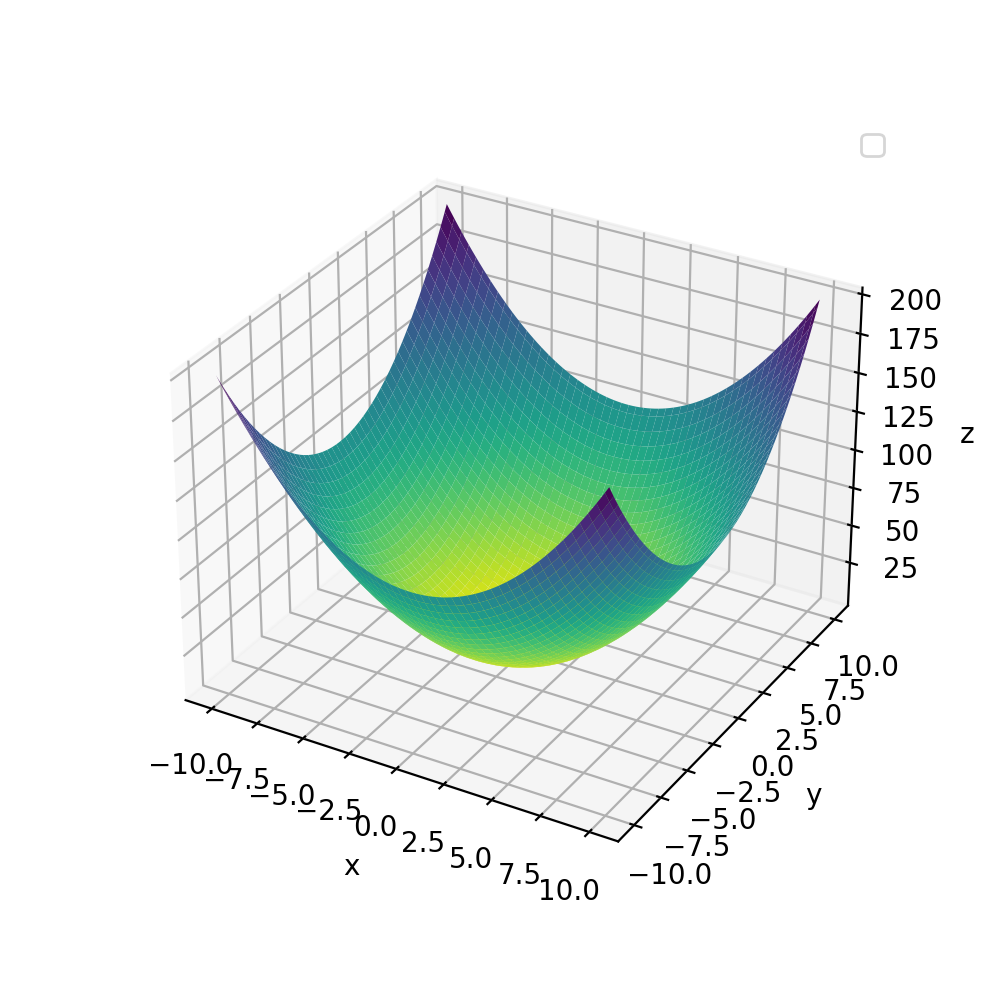
Dashboard-Plot	coming soon
2D-Plot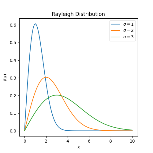

Plotly-type Plots¶

Plotting functions using via plotly.

Examples:

Python Console Session

>>> from pathlib import Path
>>> import numpy as np
>>> from umf.images.diagrams import PlotlyPlot
>>> from umf.meta.plots import GraphSettings
>>> x = np.linspace(-10, 10, 100)
>>> y = np.linspace(-10, 10, 100)
>>> X, Y = np.meshgrid(x, y)
>>> Z = X ** 2 + Y ** 2
>>> plot = PlotlyPlot(X, Y, Z, settings=GraphSettings(axis=["x", "y", "z"]))
>>> plot.plot_3d()
>>> PlotlyPlot.plot_save(plot.plot_return, Path("PlotlyPlot_3d.png"))
>>> plot.plot_contour()
>>> PlotlyPlot.plot_save(plot.plot_return, Path("PlotlyPlot_contour.png"))
>>> plot.plot_surface()
>>> PlotlyPlot.plot_save(plot.plot_return, Path("PlotlyPlot_surface.png"))

Examples:

Python Console Session

>>> from pathlib import Path
>>> import numpy as np
>>> from umf.images.diagrams import PlotlyPlot
>>> from umf.meta.plots import GraphSettings
>>> from umf.functions.distributions.continuous_semi_infinite_interval import (
...    RayleighDistribution,
... )
>>> x = np.linspace(0, 10, 100)
>>> y_sigma_1 = RayleighDistribution(x, sigma=1).__eval__
>>> y_sigma_2 = RayleighDistribution(x, sigma=2).__eval__
>>> y_sigma_3 = RayleighDistribution(x, sigma=3).__eval__
>>> plot = PlotlyPlot(
...     np.array([x, y_sigma_1]),
...     np.array([x, y_sigma_2]),
...     np.array([x, y_sigma_3]),
...     settings=GraphSettings(
...         axis=["x", r"$f(x)$"],
...         title="Rayleigh Distribution",
...     ),
... )
>>> plot.plot_series(label=[r"$\sigma=1$", r"$\sigma=2$", r"$\sigma=3$"])
>>> PlotlyPlot.plot_save(plot.plot_return, Path("PlotlyPlot_series.png"))

Parameters:

Name	Type	Description	Default
`*x`	`UniversalArray`	Input data, which can be one, two, three, or higher dimensional.	`()`
`settings`	`GraphSettings`	Settings for the graph. Defaults to None.	`None`
`**kwargs`	`dict[str, Any]`	Keyword arguments for the plot.	`{}`

plot_return property ¶

Return the plot.

check_mode(mode) ¶

Check if the mode is valid.

label_settings(*, legend=False) ¶

Set the labels for a 3D plot.

plot_2d(*, mode='lines', width=2) ¶

Plot a 2D function.

Parameters:

Name	Type	Description	Default
`mode`	`str`	The mode of the plot. Defaults to "lines".	`'lines'`
`width`	`int`	The width of the line. Defaults to 2.	`2`

plot_3d(width=2) ¶

Plot a 3D function as meshgrid.

Parameters:

Name	Type	Description	Default
`width`	`int`	The width of the line. Defaults to 2.	`2`

plot_contour(*, contours_coloring=None, showscale=False) ¶

Plot a contour plot.

Parameters:

Name	Type	Description	Default
`contours_coloring`	`str`	The color of the contours. Defaults to None.	`None`
`showscale`	`bool`	Whether to show the color scale. Defaults to False.	`False`

Raises:

Type	Description
`ValueError`	If contours_coloring is not one of "fill", "heatmap", "lines", or "none".

plot_save(fig, fname, fformat='png', scale=3, **kwargs) staticmethod ¶

Save the plot.

Parameters:

Name	Type	Description	Default
`fig`	`Figure`	The figure to save.	required
`fname`	`Path`	The filename to save the figure to.	required
`fformat`	`str`	The format to save the plot as. Defaults to "png".	`'png'`
`scale`	`int`	The scale of the plot. Defaults to 3.	`3`
`**kwargs`	`dict[str, Any]`	Additional keyword arguments to pass to the save function.	`{}`

plot_series(mode='lines', width=2, label=None) ¶

Plot a 2D function as a series.

plot_show() ¶

Show the plot.

plot_surface(*, color=None, showscale=False) ¶

Plot a 3D function as surface.

Parameters:

Name	Type	Description	Default
`color`	`str`	The color of the plot. Defaults to None.	`None`
`showscale`	`bool`	Whether to show the color scale. Defaults to False.	`False`

Types	Plotly-type Plots
3D-Plot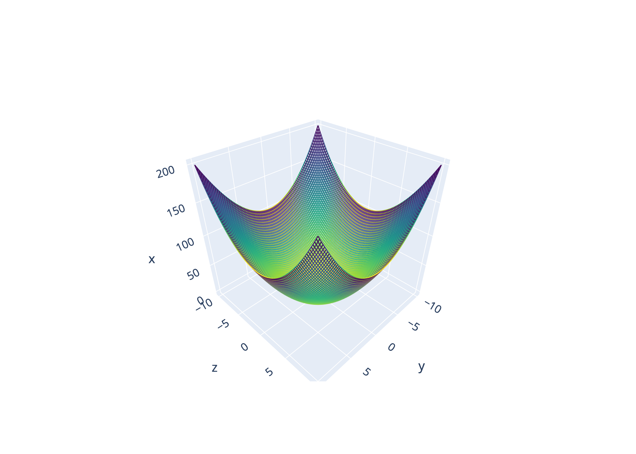
Contour-Plot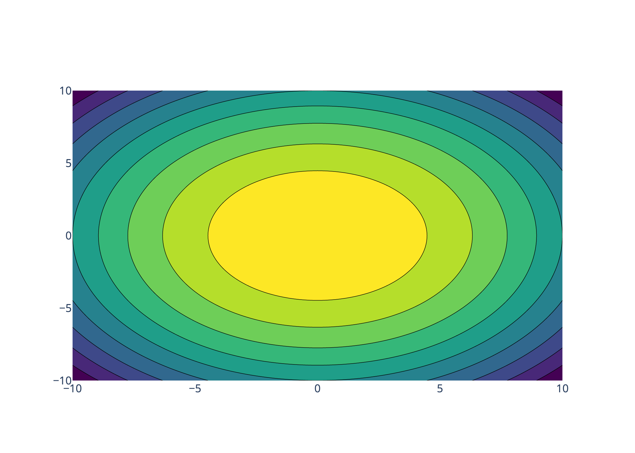
Surface-Plot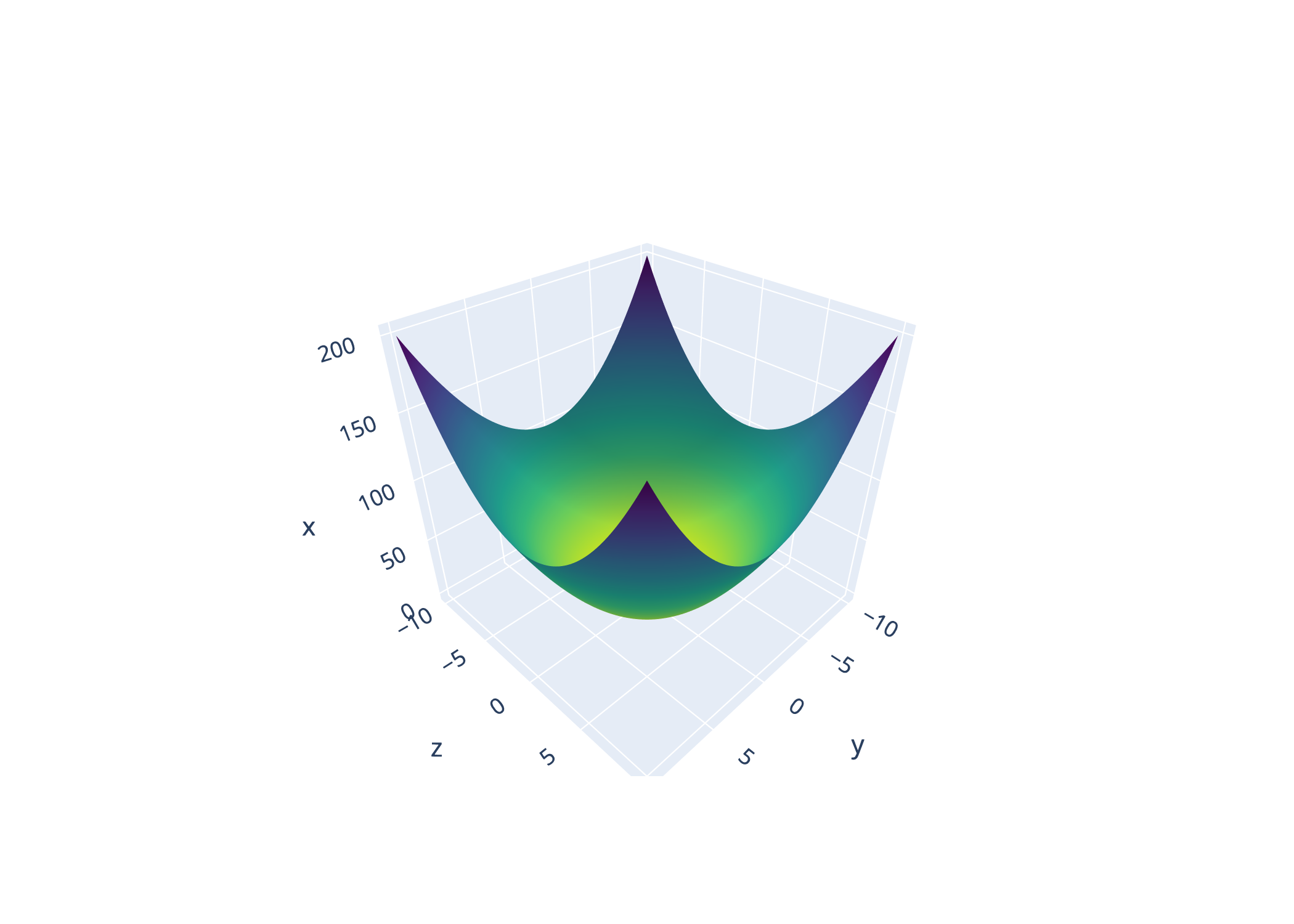
Dashboard-Plot	coming soon
2D-Plot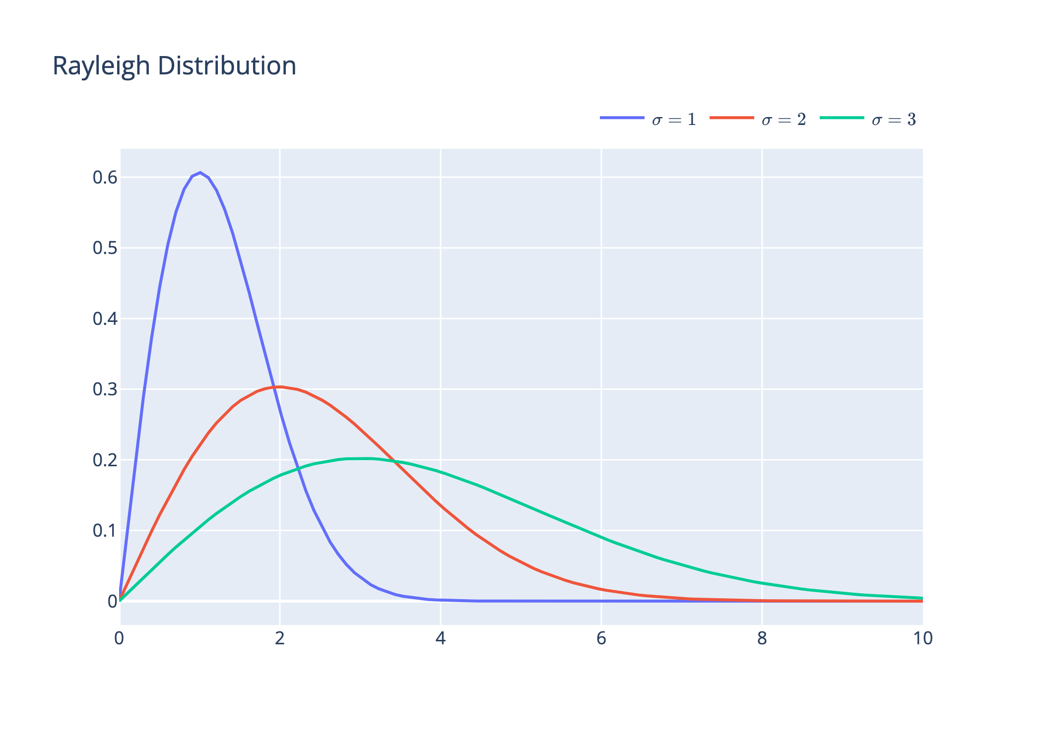